
This blog post is adapted from ex-OpenAI researcher, Anthropic co-founder Christopher Olah’s wonderful work. I removed parts that are generally commonsense to a CS kid and added some of my own notes & explanations.
Visualizing Probability Distribution
The author did a really cool job visualizing probability distribution here, but doesn’t provide any more knowledge than basic probability theory, so removed this part.
Code
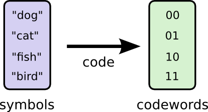
I want to communicate with my friend Bob, so we establish a code, mapping each possible word we may say to sequences of bits.
However, Bob is a dog lover, with very high probability, he talks about dogs.
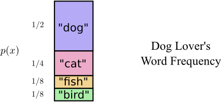
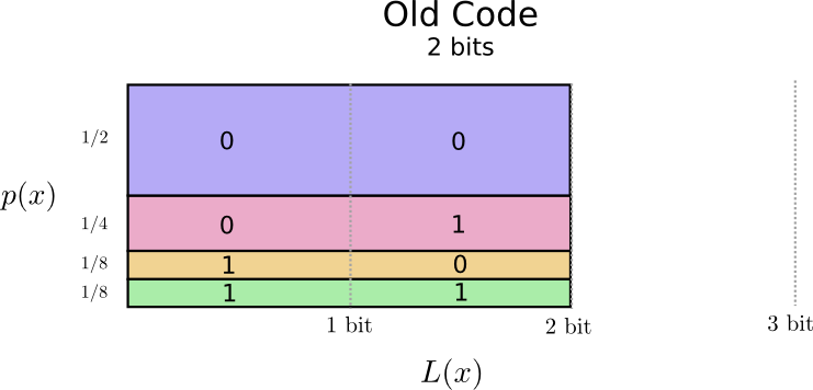
Incorporating the code we defined above into this graph, we get the following diagram, with the vertical axis to visualize the probability of each word, p(x), and the horizontal axis to visualize the length of the corresponding codeword, L(x). Notice the total area is the expected length of a codeword we send.
Variable-Length Code
Perhaps we could be very clever and make a variable-length code where codewords for common words are made especially short. The challenge is that there’s competition between codewords – making some shorter forces us to make others longer. To minimize the message length, we especially want the commonly used ones to be. So the resulting code has shorter codewords for common words (like “dog”) and longer codewords for less common words (like “bird”).
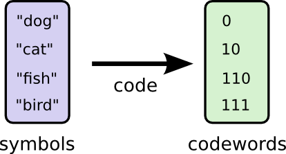
Looking at this code format with word frequency, on average, the length of a codeword is now 1.75 bits!
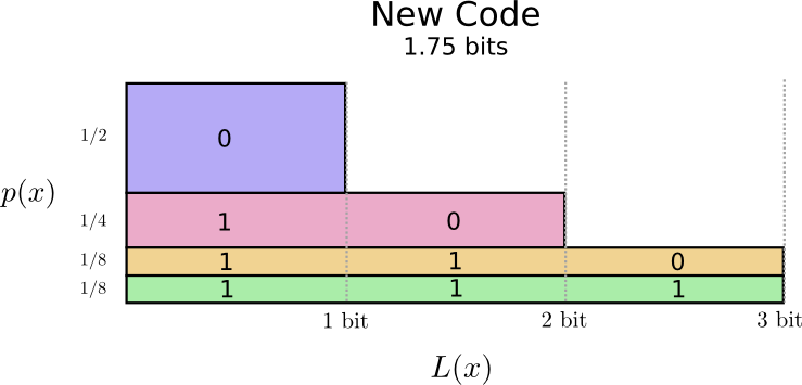
It turns out that this code is the best possible code. There is no code which, for this word frequency distribution, will give us an average codeword length of less than 1.75 bits.
There is simply a fundamental limit. Communicating what word was said, what event from this distribution occurred, requires us to communicate at least 1.75 bits on average. No matter how clever our code, it’s impossible to get the average message length to be less. We call this fundamental limit the entropy of the distribution – we’ll discuss it in much more detail shortly.
The Space of Codewords
To make our codewords uniquely decodable, we want them to follow the prefix property: no codeword should be the prefix of another codeword. i.e. If we see a particular codeword, there shouldn’t be some longer version that is also a codeword. Codes that obey this property are also called prefix codes.
One useful way to think about this is that every codeword requires a sacrifice from the space of possible codewords. If we take the codeword 01, we lose the ability to use any codewords it’s a prefix of. We can’t use 010 or 011010110 anymore because of ambiguity – they’re lost to us. The following graph shows we in effect lost $\frac {1} {2^{L(01)}} = \frac {1} {2^2} = \frac {1} {4}$ of our codeword space.
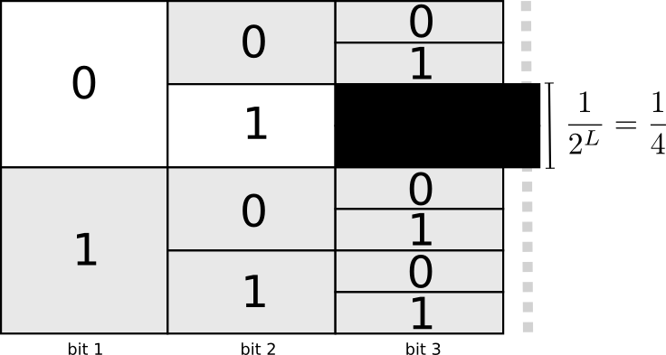
Since a quarter of all codewords start with 01, we’ve sacrificed a quarter of all possible codewords. That’s the price we pay in exchange for having one codeword that’s only 2 bits long! In turn this sacrifice means that all the other codewords need to be a bit longer. There’s always this sort of trade off between the lengths of the different codewords. A short codeword requires you to sacrifice more of the space of possible codewords, preventing other codewords from being short. What we need to figure out is what the right trade off to make is!
Cost of Codeword
You can think of this like having a limited budget to spend on getting short codewords. In fact, we have a budget = 1 to spend, where 1 is the area of the whole codeword space. We pay for one codeword by sacrificing a fraction of possible codewords.
We define the cost c of having a code word x with length L as $\frac 1 {2^{L(x)}}$.
- The cost of buying a codeword of length 0 is 1, all possible codewords – if you want to have a codeword of length 0, you can’t have any other codeword. $x = \emptyset, c = \frac 1 {2^{L(\emptyset)}} = \frac 1 {2^0}$
- The cost of a codeword of length 1, like “0”, is 1/2 because half of possible codewords start with “0”. $x = 0, c = \frac 1 {2^{L("0")}} = \frac 1 {2^1}$
- The cost of a codeword of length 2, like “01”, is 1/4 because a quarter of all possible codewords start with “01” $x = 0, c = \frac 1 {2^{L("01")}} = \frac 1 {2^2}$
- …
(ignore the gray area in the following graph, the function we plot is $\frac 1 {2^L}$ and cost is the height)
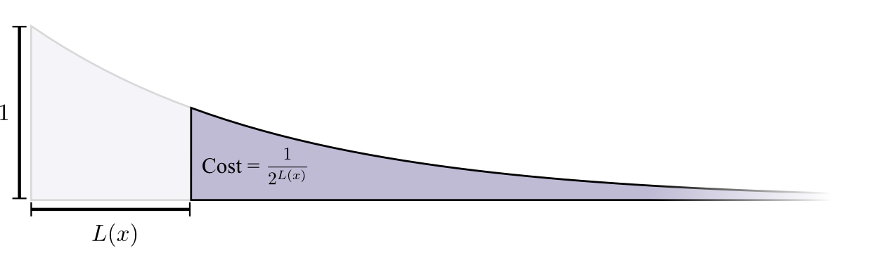
To make the calculation simpler, instead of base 2, we imagine we have the natural number e. It now is no longer a binary code, but a “natural” code with the cost becomes $\frac 1 {e^L}$. It is both the height and the gray area: $\frac 1 {e^L} = \int^\infty_L \frac 1 {e^L} \; dL$
Optimal Encoding
Recall the expected length of the codeword we pictured above, if we look at each codeword’s contribution to this expected length, each codeword makes the average message length longer by its probability times the length of the codeword. For example, if we need to send a codeword that is 4 bits long 50% of the time, our average message length is 2 bits longer than it would be if we weren’t sending that codeword. We can picture this as a rectangle.
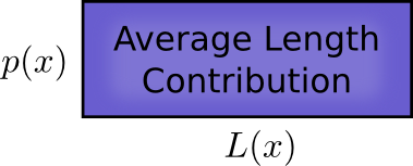
Now, we have two values related to the length of a codeword and we picture them together in the following graph:
- The amount we pay decides the length of the codeword: gray part decides the width of the purple rectangle
- The length of the codeword controls how much it adds to the average message length: width of the rec decides the area of the rec (height is fixed for a given word because height represents the word frequency)
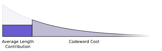
Short codewords reduce the average message length but are expensive, while long codewords increase the average message length but are cheap.
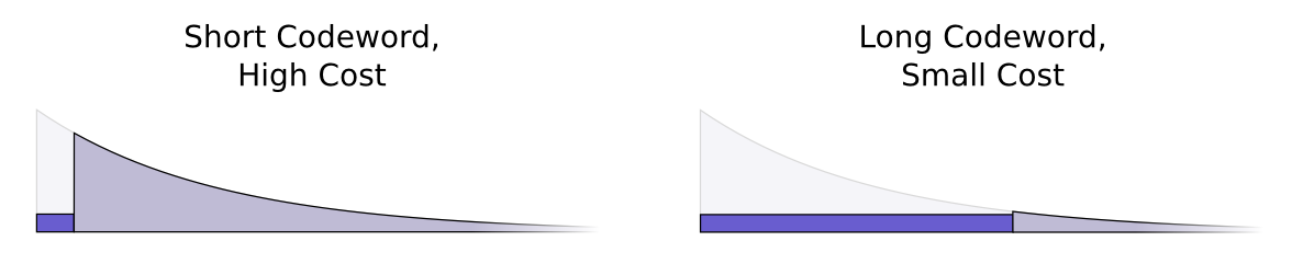
What’s the best way to use our limited budget? Just like one wants to invest more in tools that one uses regularly, we want to spend more on frequently used codewords. There’s one particularly natural way to do this: distribute our budget in proportion to how common an event is - c(x) = p(x). The following graph shows such encoding system.
Additionally, that’s exactly what we did in our codes with Bob: “dog” appears $\frac 1 2$ of the time, so we give it codeword “0” with the cost $c = \frac 1 {2^{L("0")}} = \frac 1 {2^1}$; “bird” appears $\frac 1 8$ of the time, so we give it codeword “111” with the cost $c = \frac 1 {2^{L("111")}} = \frac 1 {2^3}$; If an event only happens 1% of the time, we only spend 1% of our budget.
The author then proved it is the optimal thing to do. Honestly I didn’t understand the proof, but this code system we’re talking about here is no more than a general version of Huffman Encoding. So I guess it’s fine as long as you understand how to prove the greedy Huffman Encoding is optimal.
Calculating Entropy
In the Cost of Codeword section, we defined the cost c of having a code word x with length L as $\frac 1 {2^{L(x)}}$. By inverting this definition, given c, we can infer the length $L(x) = \log_2 \frac 1 c$
Furthermore, in the Optimal Encoding section, we proved the optimal cost to spend on each word is c(x) = p(x), so the length of the optimal encoding system is $L(x) = \log_2 \frac 1 {p(x)}$
Earlier, we said: given a probability distribution of what we want to communicate, there is a fundamental limit of expected code length we need to send no matter how smart our code is. This limit, the expected code length using the best possible code, is called the entropy of p: H(p).
$$ H(p) = \mathbb{E}_{p(x)} [L(x)] = \sum_x p(x) \log_2 \frac 1 {p(x)} $$
People usually write entropy in the following way, which makes it much less intuitive.
H(p) = −∑xp(x)log2p(x)
The entropy, which by definition is the shortest possible code, has clear implications for compression. In addition, it describes how uncertain I am and gives a way to quantify information:
- If I knew for sure what was going to happen, I wouldn’t have to send a message at all! p(x) = 1 ⟹ H(x) = 0
- If there’s two things that could happen with 50% probability, I only need to send 1 bit. ∀xi, p(xi) = 0.5 ⟹ H(x) = 1
- If there’s 64 different things that could happen with equal probability, I’d have to send 6 bits. $\forall x_i, p(x_i) = \frac 1 {64} \implies H(x) = 6$
The more concentrated the probability, the more I can craft a clever code with short average messages. The more diffuse the probability, the longer my messages have to be.
Cross Entropy
Imagine now a cat-lover Alice talks about animals with the following word frequency:
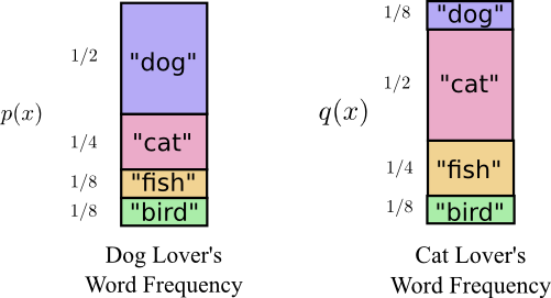
When Alice sends a message to Bob using Bob’s codes, her messages were longer than they needed to be. Bob’s code was optimized to his probability distribution. Alice has a different probability distribution, and the code is suboptimal for it: the expected codeword length when Bob uses his own code is 1.75 bits, while when Alice uses his code it’s 2.25. It would be worse if the two weren’t so similar!
The expected length of communicating an event from distribution q(x) with the optimal code for another distribution p(x) is called the cross-entropy. Formally, we define cross-entropy as: (people usually write H(q, p) instead)
$$ H_p(q) = \mathbb E_{q} \log_2\left(\frac{1}{p(x)}\right)= \sum_x q(x)\log_2\left(\frac{1}{p(x)}\right) $$
To lower the cost of Alice sending message, I asked both of them to now use Alice’s coding, but this made it suboptimal for Bob and surprisingly, it’s worse for Bob to use Alice’s code than for Alice to use his! Cross-entropy isn’t symmetric.
- Bob using his own code (H(p) = 1.75 bits)
- Alice using Bob’s code (Hp(q) = 2.25 bits)
- Alice using her own code (H(q) = 1.75 bits)
- Bob using Alice’s code (Hq(p) = 2.375 bits)
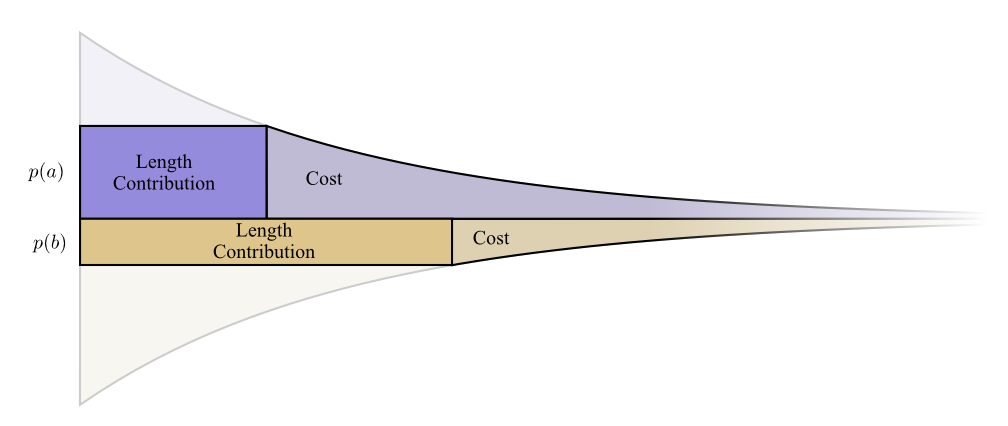
In the following diagram, if the messages are coming from the same distribution the plots are beside each other, and if they use the same codes they are on top of each other. This allows you to kind of visually slide the distributions and codes together.
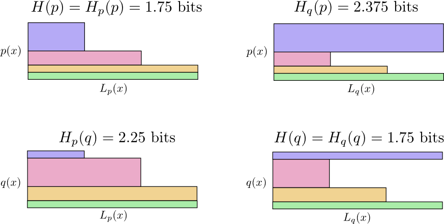
So why one is bigger than the other? This is because When Bob uses Alice’s code Hq(p), Bob says “dog” with high probability but “dog” is a word Alice happens to say the least so assigned longest length to. On the other hand for Hp(q), Bob didn’t dislike “cats” that much, so didn’t assign it with too big a word length.
KL Divergence
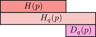
Cross-entropy gives us a way to express how different two probability distributions are. When using q’s codewords for p’s distribution, the more different the distributions p and q are, the bigger the difference is between cross-entropy of p with respect to q and the entropy of p. In math, Dq(p) = Hq(p) − H(p) is bigger.
Similarly when using p’s codewords for q’s distribution.
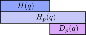
The really interesting thing is the difference Dq(p). That difference is how much longer our messages are because we used a code optimized for a different distribution q. If the distributions are the same, this difference will be zero. As the difference grows, it will get bigger.
This difference is the Kullback–Leibler divergence, or just the KL divergence. The really neat thing about KL divergence is that it’s like a distance between two distributions. It measures how different they are! (If you take that idea seriously, you end up with information geometry)
People usually write it as DLK(p||q), but our more intuitive way writes:
Dq(p) = Hq(p) − H(p)
If you expand the definition of KL divergence, you get:
$$ \begin{align} D_q(p) &= \sum_x p(x)\log_2\left(\frac{p(x)}{q(x)} \right) \\ &= \sum_x p(x) \left[ \log_2\left(\frac{1}{q(x)} \right) - \log_2\left(\frac{1}{p(x)} \right)\right]\\ &= \sum_x p(x) \left[ L_q(x) - L_p(x)\right] \end{align} $$
And we see the $\log_2\left(\frac{p(x)}{q(x)} \right)$ is simply the difference between how many bits a code optimized for q and a code optimized for p would use to represent x. The expression as a whole is the expected difference in how many bits the two codes would use
Multiple Variables and Joint Entropy
Let’s return to our weather and clothing example from earlier. My mother, like many parents, worries that I don’t dress appropriately for the weather. So, she often wants to know both the weather and what clothing I’m wearing. How many bits do I have to send her to communicate this?
To send both pieces of information, we can flatten the probability distribution (calculate the joint probability)
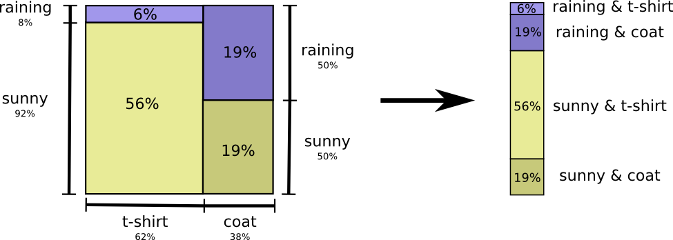
Now we can figure out the optimal codewords for events of these probabilities and compute the average message length:
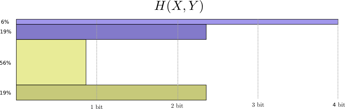
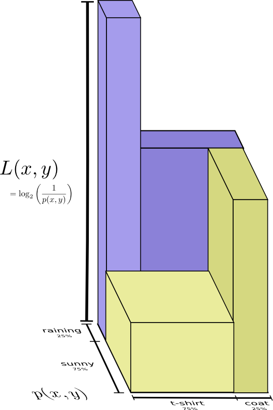
Everything is the exact same as our normal definition, except with two variables instead of one. We call this the joint entropy of X and Y, defined as
$$ H(X,Y) = \mathbb E_{p(x,y)} \log_2\left(\frac{1}{p(x,y)}\right) = \sum_{x,y} p(x,y) \log_2\left(\frac{1}{p(x,y)}\right) $$
It’s in fact more intuitive not to flatten it, but Instead to keep the 2 dimensional square and add word length as a 3rd dimension height. Now the entropy is the volume.
Conditional Entropy
Suppose my mom already knows the weather. She can check it on the news. Now how much information do I need to provide? I actually need to send less, because the weather strongly implies what clothing I’ll wear!
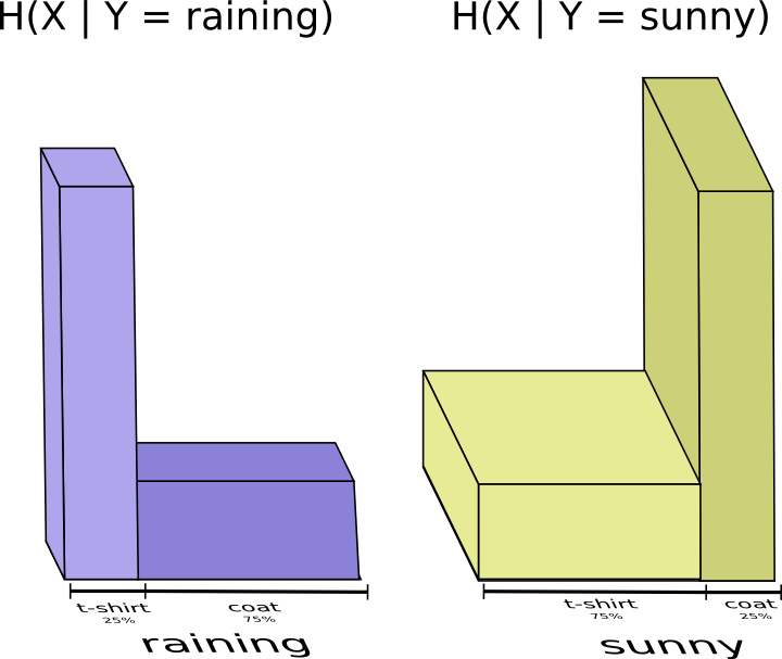
When it’s sunny, I can use a special sunny-optimized code, and when it’s raining I can use a raining optimized code. In both cases, I send less information than if I used a generic code for both. For example in case of raining, I send code length of 4 when I wear t-shirt and code length of 4/3 when I wear coat.
$$ H(X \mid \text{Y = raining}) = \frac 1 4 \log_2 \frac 1 4 + \frac 3 4 \log_2 \frac 3 4 = 0.81 $$
(Don’t worry for now why the entropy, representing length of an optimal codeword, can be fractional, we will explain it later)
With a similar calculation, we show H(X ∣ Y = sunny) = 0.81. To get the average amount of information I need to send my mother, I just put these two cases together:
$$ \begin{align} H(X \mid Y) &= P(\text{Y = rainy})\,H(X \mid \text{Y = rainy})+ P(\text{Y = sunny})\,H(X \mid \text{Y = sunny}) \\ &= \frac 1 4 \times 0.81 + \frac 3 4 \times 0.81 = 0.81 \end{align} $$
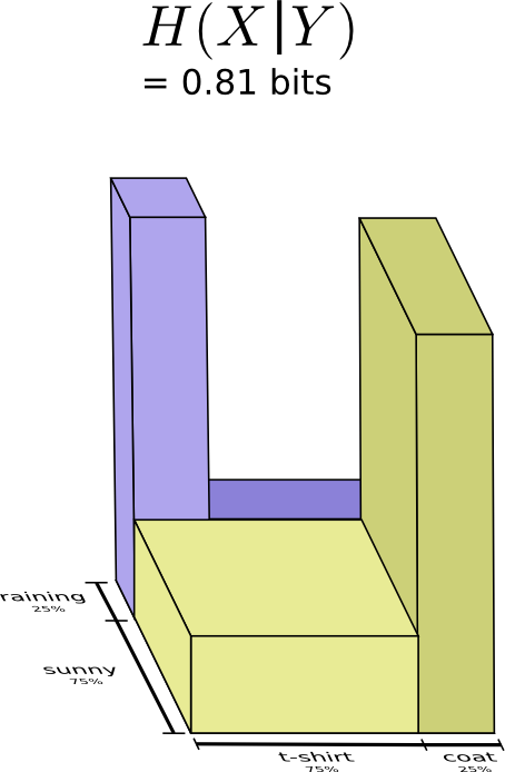
We call this the conditional entropy:
$$ \begin{align} H(X|Y) &= \sum_y p(y) H(X \mid Y=y) \\ &= \sum_y p(y) \sum_x p(x|y) \log_2\left(\frac{1}{p(x|y)}\right) \\ &= \sum_{x,y} p(x,y) \log_2\left(\frac{1}{p(x|y)}\right) \end{align} $$
Mutual Information
In the previous section, we observed that knowing one variable can mean that communicating another variable requires less information.
One nice way to think about this is to imagine amounts of information as bars. These bars overlap if there’s shared information between them: some of the information in X and Y is shared between them, so H(X) and H(Y) are overlapping bars. And since H(X, Y) is the information in both, it’s the union of the bars H(X) and H(Y).
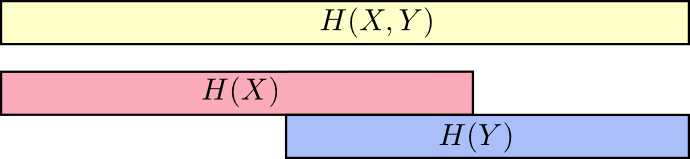
We rank the information needed to communicate these 3 kinds of things in descending order:
- Both X and Y: joint entropy H(X, Y)
- X alone: marginal entropy H(X)
- X when Y is known: conditional entropy H(X|Y)

In the bar perspective, H(X|Y) is the information we need to send to communicate X to someone who already knows Y - it is the information in X which isn’t also in Y. Visually, that means H(X|Y) is the part of H(X) bar which doesn’t overlap with H(Y).
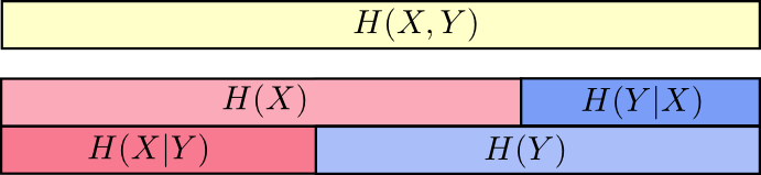
From this, we get another identity: the information in X and Y is the information in Y plus the information in X which is not in Y. (sounds like set, doesn’t it?)
H(X, Y) = H(Y) + H(X|Y)
To wrap up, we have
- information in each variable: H(X) and H(Y)
- union of the information in both: H(X, Y)
- information in one but not the other: H(X|Y) and H(Y|X)
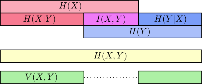
We can further define mutual information: information both in X and Y, or in set terms, the intersection of information:
I(X, Y) = H(X) + H(Y) − H(X, Y)
If you expand the definition of mutual information out, you get:
$$ I(X,Y) = \sum_{x,y} p(x,y) \log_2\left(\frac{p(x,y)}{p(x)p(y)} \right) $$
That looks suspiciously like KL divergence!
Well, it is KL divergence. It’s the KL divergence of P(X, Y) and its naive approximation P(X)P(Y). That is, it’s the number of bits you save representing X and Y if you understand the relationship between them instead of assuming they’re independent.
and the variation of information. The variation of information is the information which isn’t shared between the variables. It gives a metric of distance between different variables. The variation of information between two variables is zero if knowing the value of one tells you the value of the other and increases as they become more independent.
V(X, Y) = H(X, Y) − I(X, Y)
How does this relate to KL divergence, which also gave us a notion of distance? Well, KL divergence gives us a distance between two distributions over the same variable or set of variables. In contrast, variation of information gives us distance between two jointly distributed variables. KL divergence is between distributions, variation of information within a distribution.
In summary, we put them all in a single diagram:
Fractional Bits
A careful reader may have noticed that in previous calculations, we had fractional length of message. Isn’t that weird? How should we interpret such a message? How is it done in real life?
The answer is: you can think of them as expected length of a message. If half the time one sends a single bit, and half the time one sends two bits, on average one sends one and a half bits. There’s nothing strange about averages being fractional.
That’s a quick but vague answer. Let’s look at an example: consider a probability distribution where one event a happens 71% of the time and another event b occurs 29% of the time.
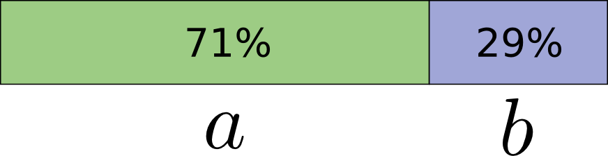
The optimal code would use 0.5 bits to represent a, and 1.7 bits to represent b. Well, if we want to send a single one of these codewords, it simply isn’t possible. We’re forced to round to a whole number of bits, and send on average 1 bit.
… But if we’re sending multiple messages at once, it turns out that we can do better. Let’s consider communicating two events from this distribution. If we send them independently, using the code we established for a single event, we’d need to send two bits. Can we do better?
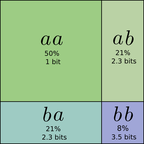
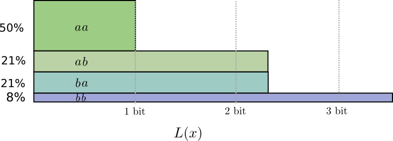
Half the time, we need to communicate aa, 21% of the time we need to send ab or ba, and 8% of the time we need to communicate bb. Again, the ideal code involves fractional numbers of bits.
If we round the codeword lengths, we’ll get something like this:
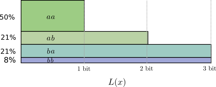
This codes give us an average message length of 1.8 bits. That’s less than the 2 bits when we send them independently. Another way of thinking of this is that we’re sending 1.8/2 = 0.9 bits on average for each event. If we were to send more events at once, it would become smaller still. As n tends to infinity, the overhead due to rounding our code would vanish, and the number of bits per codeword would approach the entropy.
Further, notice that the ideal codeword length for a was 0.5 bits, and the ideal codeword length for aa was 1 bit. Ideal codeword lengths add, even when they’re fractional! So, if we communicate a lot of events at once, the lengths will add.
Conclusion
- Entropy is optimal length ..
- KL divergence ..
- Entropy over multiple variables can be interpreted as sets of information