Decision Tree

Motivation for Decision Trees¶

Recall the kD tree data structure. Decision trees also divide the data into different regions, except that it stops dividing when current region is pure (all have the same label). Therefore, if a test point falls into any bucket, we can just return the label of that bucket. Our new goal becomes to build a tree that is:

1. Maximally compact (of minimal size)
2. Only has pure leaves

Finding such a minimum size tree turns out to be NP-Hard. But the good news is: We can approximate it very effectively with a greedy strategy. We keep splitting the data to minimize an impurity function that measures label purity amongst the children.

Impurity Functions¶

Data: $S=\left\{ \left( \mathbf{x}_1,y_1 \right),\dots,\left( \mathbf{x}_n,y_n \right) \right\}, y_i\in \left\{ 1,\dots,c \right\}$, where $c$ is the number of classes.

Let $S_k\subseteq S$ be the inputs with labels $k$. Formally, $S_k=\left \{ \left ( \mathbf{x},y \right )\in S:y=k \right \}$, so $S=S_1\cup \dots \cup S_c$. Define

We know what we don’t want (Uniform Distribution): $p_1=p_2=\dots=p_c=\frac{1}{c}$. This is the worst case since each class is equally likely. Making decision based on some algorithm is no better than random guessing.

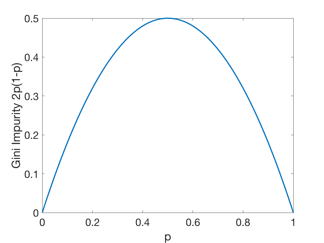
Gini impurity¶

So Gini impurity on a leaf is:

Fig: The Gini Impurity Function in the binary case reaches its maximum at $p=0.5$

This corresponds with the idea that uniform distribution is the least we want to see.

Gini impurity of a tree is:

Entropy¶

Define the impurity as how close we are to uniform. Use $KL$-Divergence to describe “closeness” from $p$ to $q$. (Note: $KL$-Divergence is not a metric because it is not symmetric, i.e. $KL(p||q)\neq KL(q||p)$)

In our case, $p$ is our distribution and let $q_1,\dots,q_c$ be the uniform label/distribution. i.e. $\forall k, \; q_k=\frac{1}{c}$. We will calculate the KL divergence between $p$ and $q$.

If we are uniform (our least wanted case), $\log \frac {p_k} {q_k} = \log 1 = 0$, so $KL = 0$. From this, we see that at the end we want to maximize the distance $KL$.

Since $log(c)$ is constant and $\sum_{k}p_k=1$,

Define entropy of set $S$ is $H(s) = -\sum_{k}p_klog(p_k)$. We have therefore translated the problem of maximizing distance to minimizing entropy.

Entropy on a tree is defined the same as Gini impurity.

ID3-Algorithm¶

Base Cases¶

In two situations, we say that we have reached the base case:

1. there is no need to split: all the data points in a subset have the same label, so return that label
2. there is no way to split: there are no more attributes could be used to split the subset (all the data points have the same value across all entries), so return the most common label

Note, we do not stop when if no split can improve impurity:

Why? Look at the following XOR example

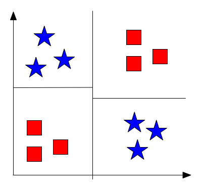
Decision trees are myopic: ID3 (and possibly all algorithms used to find decision trees) is a greedy algorithm and only looks at one feature at a time. In the example, the first split does NOT decrease the impurity measure, however, if combining two feature splits, we reduce the impurity measure to 0.

Recursion Step and Time Analysis¶

At each recursion, we find the split that would minimize impurity based on these two parameters:

• $f$ - the feature to use
• $t$ - threshold (where to draw the line)

For a specific feature/dimension $i$, there are $n-1 = O(n)$ possible places to draw the line (the same as putting dividers between balls). When we draw such a line at $t$, we are basically dividing the set into $x_f\le t$ and $x_f \gt t$, so

To draw such a line based on dimension $i$, we first have to sort all data points by $x_i$ - their value on this dimension. This sort takes $O(n\;\log n)$ time and we need test all $O(n)$ possible line positions to determine where to draw the line. Therefore, it takes $O(n\;\log n)$ time for each feature.

For all features and all corresponding places to draw the line, choose the division that minimizes impurity function. There are a total $d$ features, so each final drawing takes

Regression Trees - CART¶

CART stands for Classification and Regression Trees.

Assume labels are continuous: $y_i\in\mathbb{R}$, we can just use squared loss as our impurity function, so

This model has the following characteristics:

• CART are very light weight classifiers
• Very fast during testing
• Usually not competitive in accuracy but can become very strong through bagging (Random Forests) and boosting (Gradient Boosted Trees)

Parametric vs. Non-parametric algorithms¶

So far we have introduced a variety of algorithms. One can categorize these into different families, such as generative vs. discriminative, or probabilistic vs. non-probabilistic. Here we will introduce another one: parametric vs. non-parametric.

• A parametric algorithm is one that has a constant set of parameters, which is independent of the number of training samples. You can think of it as the amount of much space you need to store the trained classifier. An examples for a parametric algorithm is the Perceptron algorithm, or logistic regression. Their parameters consist of $\mathbf{w},b$, which define the separating hyperplane. The dimension of $\mathbf{w}$ depends on the dimension of the training data, but not on how many training samples you use for training.
• In contrast, the number of parameters of a non-parametric algorithm scales as a function of the number of training samples. An example of a non-parametric algorithm is the $k$-Nearest Neighbors classifier. Here, during “training” we store the entire training data -- so the parameters that we learn are identical to the training set and the number of parameters (/the storage we require) grows linearly with the training set size.

Decision Tree is an interesting edge case. If they are trained to full depth they are non-parametric, as the depth of a decision tree scales as a function of the training data (in practice $O(\log_2(n))$). If we however limit the tree depth by a maximum value they become parametric (as an upper bound of the model size is now known prior to observing the training data).