Boosting

Generic Boosting¶

Boosting Reduces Bias¶

Scenario: Hypothesis class $\mathbb{H}$, whose set of classifiers has large bias and the training error is high (e.g. CART trees with very limited depth.)

Famous question: Can weak learners ($h$) be combined to generate a strong learner with low bias?

Answer: Yes!

Solution: Create ensemble classifier $H_T(\vec x) = \sum_{t = 1}^{T}\alpha_t h_t(\vec{x})$. This ensemble classifier is built in an iterative fashion. In iteration $t$ we add the classifier $\alpha_th_t(\vec x)$ to the ensemble. At test time we evaluate all classifier and return the weighted sum.

Let $\ell$ denote a (convex and differentiable) loss function.

Assume we have already finished $t$ iterations and already have an ensemble classifier $H_t(\vec{x})$. Now at iteration $t+1$ we add one more weak learner $h_{t+1}$ that minimizes the loss:

So $H_{t+1} := H_t + \alpha h$

Finding $h$ - Gradient Descent in Functional Space¶

As before, we find minimum by doing gradient descent. However, instead of finding a parameter that minimizes the loss function, we find a function $h$ this time. Therefore we will do gradient descent in function space.

Given $H$, we want to find the step-size $\alpha$ and the weak learner $h$ to minimize the loss $\ell(H+\alpha h)$. Use Taylor Approximation on $\ell(H+\alpha h)$:

This approximation only holds within a small region around $\ell(H)$. We therefore fix $\alpha$ to a small constant (e.g. $\alpha\approx 0.1$). With the step-size $\alpha$ fixed, we can use the approximation above to find an almost optimal $h$:

$$

$$

In function space, inner product is defined as $< f,g >=\int\limits_x f(x)g(x)dx$. This is intractable most of the time because $x$ comes from an infinite space. Since we only have training set, we can rewrite the inner product as $< f,g >= \sum_{i = 1}^{n} f(\mathbf{x}_i)g(\mathbf{x}_i)$, where $f$ is the gradient, $g$ is model $h$.

Note $\frac{\partial \ell}{\partial H}$ is the derivative of a function with respect to another function, which is tricky, so we need a work-around. $\ell(H) = \sum_{i = 1}^{n}\ell(H(\mathbf{x}_i))$, so we can write $\frac{\partial \ell}{\partial H}(\mathbf{x}_i) = \frac{\partial \ell}{\partial [H(\mathbf{x}_i)]}$, the derivative of the loss with respect to a specific function value. Now the optimization problem becomes:

In order to make progress this $h$ does not have to be great (reach a minimum). We still make progress as long as $\sum_{i = 1}^{n} r_i h(\mathbf{x}_i)<0$. That is because

In this way, we decrease the loss by adding this new model $h_{t+1}$. However, if the this inner product is >0 there is nothing we can do with gradient descent.

Generic boosting (a.k.a Anyboost) in Pseudocode¶

注意，下图只是把我们上一节描述的东西用伪代码写下来了而已，实际是完全一样的东西。

Case study #1: Gradient Boosted Regression Tree(GBRT)¶

Background and Setting¶

• Classification ($y_i \in \{+1,-1\}$) or regression ($y_i\in\mathcal{R}^k$)
• Weak learners,$h \in \mathbb{H}$, are not too deep fixed-depth (e.g. depth=4) regression trees .
• Step size $\alpha$ is fixed to a small constant (hyper-parameter).
• Loss function: Any differentiable convex loss that decomposes over the samples $\mathcal{L}(H)=\sum_{i=1}^{n} \ell(H(\mathbf{x}_i))$

Goal¶

We want to find a tree $h$ that maximizes $h = \textrm{argmin}_{h \in \mathbb{H}} \sum_{i = 1}^{n} r_i h(\mathbf{x}_i)$ where $r_i = \frac{\partial \ell}{\partial H(\mathbf{x}_i)}$.

Assumptions¶

1. First, we assume that $\sum_{i = 1}^{n} h^2(\mathbf{x}_i)$ = constant. So we are essentially fixing the vector $h$ in $\sum_{i=1}^n h(\mathbf{x}_i)r_i$ to lie on a circle, and we are only concerned with its direction but not its length.
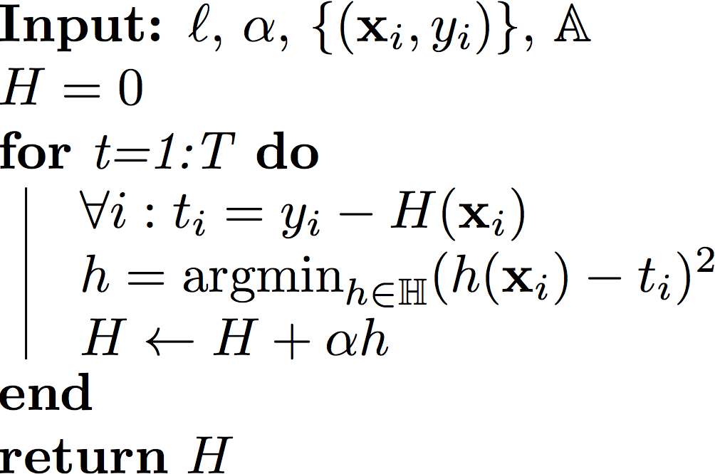
2. Define the negative gradient as $t_i = -r_i = -\frac{\partial \ell}{\partial H(\mathbf{x}_i)}$.

Algorithm¶

At the second last step, note $t_i^2$ is the negation of loss function with respect to the ensemble $H$ we already chose, independent of the model $h$ we are choosing, so it is a constant. On the other hand, we constrained in the assumptions part that $\sum_{i = 1}^{n} h^2(\mathbf{x}_i)$ is a constant.

Therefore, we translate the original problem about finding a regression tree that minimizes an arbitrary loss function to this problem of finding a regression tree that minimizes the squared loss with our new “label” $t$ and we are fitting $t$ now.

If the loss function $\ell$ is the squared loss, i.e. $\ell(H)=\frac{1}{2}\sum_{i=1}^n (H(\mathbf{x}_i)-y_i)^2$, there is a special meaning of this $t$: it is easy to show that

which is simply the error between our current prediction and the correct label, so this newly added model is just fitting the error current ensemble model has. However, it is important to keep in mind that you can use any other differentiable and convex loss function $\ell$ and the solution for your next weak learner $h$ will always be the regression tree minimizing the squared loss.

GBRT in Pseudo Code¶

Case Study #2: AdaBoost¶

• Setting: Classification ($y_i \in \{+1,-1\}$)
• Step-size: We perform line-search to obtain best step-size $\alpha$.
• Loss function: Exponential loss $\ell(H)=\sum_{i=1}^{n} e^{-y_i H(\mathbf{x}_i)}$
• All data points must have the correct label, since we are using the exponential loss here and will get a very bad result if concentrate all our weights on noise (wrongly labeled data).

Finding the best weak learner¶

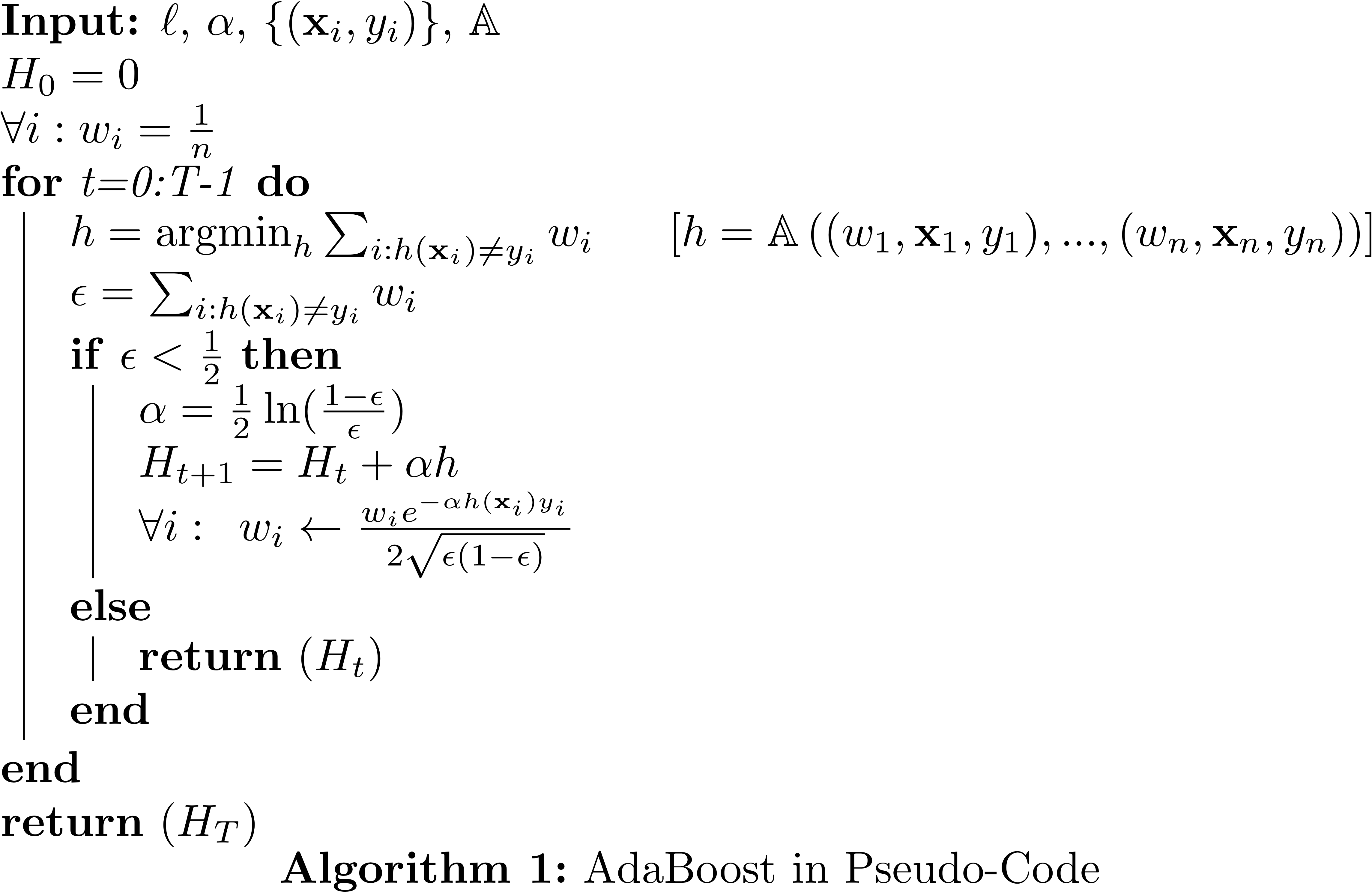
At each update step, first we compute the gradient $r_i=\frac{\partial \ell}{\partial H(\mathbf{x}_i)}=-y_i {e^{-y_i H(\mathbf{x}_i)}}$. For notational convenience, define $w_i= \frac{1}{Z}e^{-y_iH(\mathbf{x}_i)}$, where $Z=\sum_{i=1}^{n} e^{-y_iH(\mathbf{x}_i)}$ is a normalizing factor so that $\sum_{i=1}^{n} w_i=1.$ Note that the normalizing constant $Z$ is identical to the loss function. Each weight $w_i$ can now be interpreted as the relative contribution of the training point $(\mathbf{x}_i,y_i)$ towards the overall loss. Therefore, at each update step, we reweight the data points according to current loss and in later part of the algorithm will prioritize those points we got really wrong.

We can translate the optimization problem of minimizing loss into a optimization probelm of minimizing the weighted classification error.

Let us denote this weighted classification error as $\epsilon=\sum_{i:h(\mathbf{x}_i)y_i=-1} w_i$, or to say the weights of those wrongly classified points. So for AdaBoost, we only need a classifier that reduces this weighted classification error of these wrongly labeled training samples. It doesn’t have to do all that well, in order for the inner-product $\sum_i r_i h(\mathbf{x}_i)$ to be negative, it just needs less than $\epsilon<0.5$ weighted training error.

Finding the stepsize $\alpha$¶

In the previous example, GBRT, we set the stepsize $\alpha$ to be a small constant. As it turns out, in the AdaBoost setting we can find the optimal stepsize (i.e. the one that minimizes $\ell$ the most) in closed form every time we take a “gradient” step.

If we take the derivative of loss function $\ell$ with respect to $\alpha$, we will actually find out that there is a nice closed form for $\alpha$:

It is unusual that we can find the optimal step-size in such a simple closed form. One consequence is that AdaBoost converges extremely fast.

Re-normalization¶

After you take a step, i.e. $H_{t+1}=H_{t}+\alpha h$, you need to re-compute all the weights and then re-normalize. However, if we update $w$ using the formula below, $w$ will remain normalized.

AdaBoost Pseudo-code¶

The inner loop can terminate as the error $\epsilon=\frac{1}{2}$, and in most cases it will converge to $\frac{1}{2}$ over time. In that case the latest weak learner $h$ is only as good as a coin toss and cannot benefit the ensemble (therefore boosting terminates). Also note that if $\epsilon=\frac{1}{2}$ the step-size $\alpha$ would be zero.

Further analysis¶

We can in fact show that the training loss is decreasing exponentially! Even further, we can show that after $O(\log(n))$ iterations your training error must be zero. In practice it often makes sense to keep boosting even after you make no more mistakes on the training set.