Back Propagation

Reverse Mode Automatic Differentiation¶

We need to fix an output in the NN. For most cases, we just use the final output $\ell$ of the NN ($\ell$ stands for loss). For each intermediate output value $y$, we want to compute partial derivatives $\frac{\partial \ell}{\partial y}$.

Same as before: we replace each number/array $y$ with a pair, except this time the pair is not $(y, \frac{\partial y}{\partial x})$ but instead $(y, \nabla_y \ell)$ where $\ell$ is our final output (loss of NN). Observe that $\nabla_y \ell$ always has the same shape as $y$.

Deriving Backprop from the Chain Rule¶

Single Variable¶

Suppose that the output $\ell$ can be written as

Here, $g$ represents the immediate next operation that takes $y$ (producing a new intermediate $u$), and $f$ represents all the rest of the computation between $u$ and $\ell$. By the chain rule,

Therefore, to compute $\frac{\partial \ell}{\partial y}$, in addition to $\frac{\partial \ell}{\partial u}$ - the derivative of all the other intermediate computation, we only need to use “local” information $g'(y)$ that’s available in the program around where $y$ is computed and used. That is, if ignore $\frac{\partial \ell}{\partial u}$, we can compute $\frac{\partial \ell}{\partial y}$ together when we compute $y$.

Multi Variable¶

More generally, suppose that the output $\ell$ can be written as

Here, the $g_1, g_2, \ldots, g_k$ represent the immediate next operations that take $y$; the $u_i$ are the output by these operations, and $F$ represents all the rest of the computation between $u$ and $\ell$. By the multivariate chain rule,

Note here we are talking about the more general case, where $\ell, u, y$ are all vectors. So $g_i$ takes in a vector $y$ and outputs a vector $u_i$ When we take the derivative of $g_i$ at $y$, we get a matrix and we call this matrix $D g_i(y)$

Again, we see that we can compute $\nabla_y \ell$ using only $\nabla_{u_i} \ell$ and “local” information $D g_i(y)$.

Computing Backprop¶

When to Compute?¶

Note the $\ell$ value is computed as follows: $y \to u \to \ell$ So when we are computing $y$ , which is also when we ideally want to compute $\frac{\partial \ell}{\partial y}$, the value of $u$ is not yet available. Without $u$, we cannot compute $\frac{\partial \ell}{\partial u}$, which is a necessary part to get $\frac{\partial \ell}{\partial y}$. Therefore we cannot compute $\frac{\partial \ell}{\partial y}$ along with $y$

Therefore, we cannot compute $\frac{\partial \ell}{\partial y}$ until after we’ve computed everything between $y$ and $\ell$. So the solution is to remember the order in which we computed stuff in between $y$ and $\ell$, and then compute their gradients in the reverse order.

Computational Graph¶

We draw a graph to indicate the computational dependencies, just like the $y \to u \to \ell$ above:

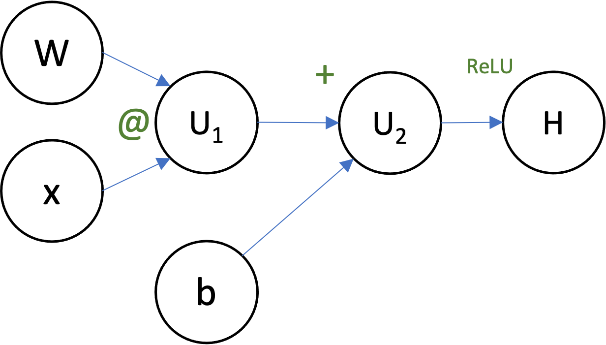
• node represents an scalar/vector/tensor/array
• Edges represent dependencies, where $y \rightarrow u$ means that $y$ was used to compute $u$

Algorithm¶

Generally speaking,

1. For each tensor, initialize a gradient “accumulator” to 0. Set the gradient of $\ell$ with respect to itself to 1.

2. For each tensor $y'$ that $\ell$ depends on, in the reverse order of computation, compute $\nabla_{y'} \ell$ - derivative of $\ell$ with respect to $y'$. This is obtainable because when we get to $y'$, all the intermediate value $u$ between $y'$ and $\ell$ are already computed.

   Once this step is called for $y$, its gradient will be fully manifested in its gradient accumulator.

In a computational graph, this means

1. For each tensor, initialize a gradient “accumulator” to 0. Set the gradient of $\ell$ with respect to itself to 1.

2. For each tensor $y'$ pointing to $\ell$, start from $\ell$ and go back along the path, compute $\nabla_{y'} \ell$ - derivative of $\ell$ with respect to $y'$. Specifically, we compute this value by looking at all its direct descendants $u_i$ where $\nabla_{y'} \ell = \sum_{i=1}^k \frac{\partial \ell}{\partial u_i} \frac{\partial u_i}{\partial y'}$ We can do this because $u$ are the nodes between $y'$ and $\ell$, when we get to $y'$, all $u$ values are already computed.

   Once this step is called for $y$, computation is done.