K-Nearest Neighbors

The k-NN algorithm¶

Assumption: Similar inputs have similar outputs / Similar points have similar labels.

Classification rule: For a test input $\mathbf{x}$, assign the most common label amongst its k most similar training inputs

Formal Definition:

For a point $\mathbf{x}$, denote the set of the $k$ nearest neighbors of $\mathbf{x}$ as $S_\mathbf{x}$. Formally, $S_\mathbf{x}\subseteq {D}$ s.t. $|S_\mathbf{x}|=k$ and $\forall(\mathbf{x}',y')\in D\backslash S_\mathbf{x}, \text{dist}(\mathbf{x},\mathbf{x}')\ge\max_{(\mathbf{x}'',y'')\in S_\mathbf{x}} \text{dist}(\mathbf{x},\mathbf{x}'')$

Classifier $h(\mathbf{x})$ takes in a test point and returns the most common label in $S_\mathbf{x}$:

How does $k$ affect the classifier?

As k $\uparrow$, decision boundary gets smoother. When $k=n$, we always output $mode\{D\}$; if $k =1$, we always output test point’s nearest point.

What distance function should we use?¶

The k-nearest neighbor classifier fundamentally relies on a distance metric. The better that metric reflects label similarity, the better the classified will be. The most common choice is the Minkowski distance:

• $p = 1$: Absolute Value / Manhattan Distance
• $p = 2$: Euclidian Distance
• $p \to \infty$: Max (其他项都会被最大项的 $|x_r-z_r|^p$ 给 shadow 掉，再取 $...^{1/p}$ 回到 $|x_r-z_r|$)

Brief digression: Bayes optimal classifier¶

Assume (and this is almost never the case) we have all knowledge about the distribution. That is we know $P(X,Y)$, the distribution from which our samples are drawn. we can then get every value we want. For example, if we want to have $\mathrm{P}(y|\mathbf{x})$ we just have to use the Bayes rule and calculate $\frac{P(\mathbf{x},y)}{P(\mathbf{x})}$, where $P(\mathbf{x}) = \int_{y'} P(\mathbf{x},y')$.

Therefore, if we know this ultimate distribution, which gives us $\mathrm{P}(y|\mathbf{x})$, then you would simply predict the most likely label:

即我们已知对于每个输入 x，输出各个 y 的可能性，那么给一个 x 只需输出最可能的 y 即可

Although the Bayes optimal classifier is as good as it gets, it still can make mistakes. It is always wrong if a sample does not have the most likely label. We can compute the probability of that happening precisely (which is exactly the error rate):

Assume for example an email $\mathbf{x}$ can either be classified as spam $(+1)$ or ham $(-1)$. For the same email $\mathbf{x}$ the conditional class probabilities are:

In this case the Bayes optimal classifier would predict the label $y^*=+1$ as it is most likely, and its error rate would be $\epsilon_{BayesOpt}=0.2$. 也就是说，有0.2的邮件即使看起来很像 spam 但它们并不是 spam

Bayes optimal classifier is an lower bound on error: no model can do better than the Bayes optimal classifier.

We also have constant classifier as an upper bound on error: constant classifier always predicts the same constant - most common label in the training set (equivalent to a KNN with $k = n$). Your model should always do better than the constant classifier.

1-NN Convergence Proof¶

Cover and Hart 1967[1]: As $n \to \infty$, the 1-NN error is no more than twice the error of the Bayes Optimal classifier. (Similar guarantees hold for $k>1$.)

$n$ small	$n$ large	$n\to\infty$

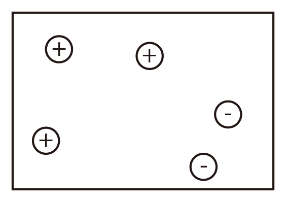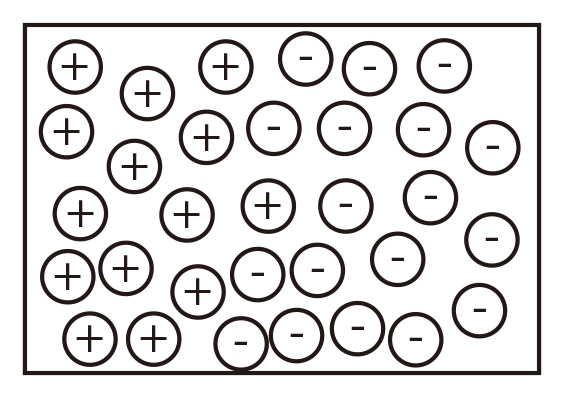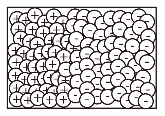Let $\mathbf{x}_\mathrm{NN}$ be the nearest neighbor of our test point $\mathbf{x}_\mathrm{t}$. As $n \to \infty$, $\text{dist}(\mathbf{x}_\mathrm{NN},\mathbf{x}_\mathrm{t}) \to 0$, i.e. $\mathbf{x}_\mathrm{NN} \to \mathbf{x}_{t}$. (Since there are just too many points, the nearest neighbor will eventually become identical to our test point)

Since we are doing 1NN, we return the label of $\mathbf{x}_\mathrm{NN}$. Consider the error rate: the probability that label of $\mathbf{x}_\mathrm{NN}$ is not the label of $\mathbf{x}_\mathrm{t}$. This happens when test point has the most common label it should have, but NN has something else. Or when NN has the most common label it should have, but test point has something else. $$

$$where we used that$\mathrm{P}(y^* | \mathbf{x}\mathrm{t})=\mathrm{P}(y^* | \mathbf{x}\mathrm{NN})$because we have assumption:$\mathbf{x}\mathrm{NN} \to \mathbf{x}\mathrm{t}$.

Good news: As $n \to\infty$, the 1-NN classifier is only a factor 2 worse than the best possible classifier.

Bad news: We are cursed!!

Curse of Dimensionality¶

Distances between points¶

Figure demonstrating "the curse of dimensionality’'. The histogram plots show the distributions of all pairwise distances between randomly distributed points within $d$-dimensional unit squares. As the number of dimensions $d$ grows, all distances concentrate within a very small range.

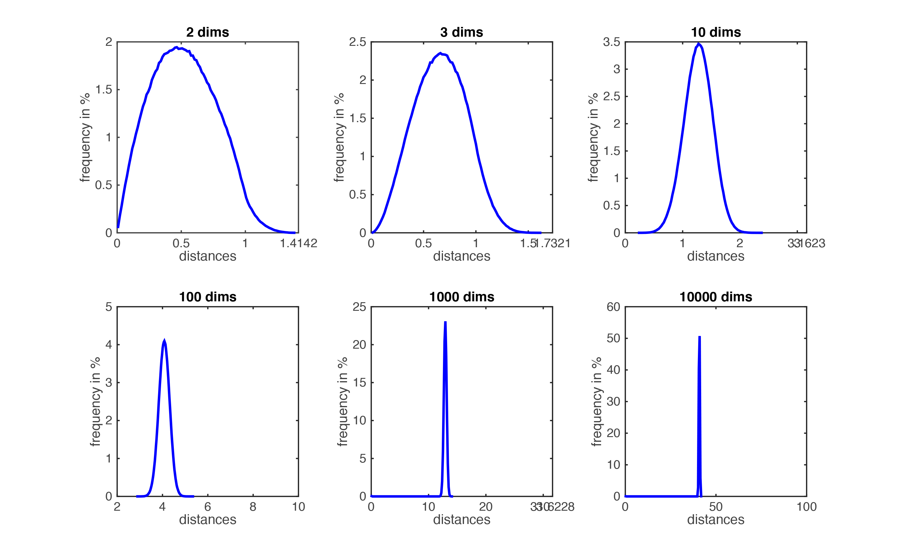
The $k$NN classifier makes the assumption that similar points share similar labels. Unfortunately, in high dimensional spaces, points that are drawn from a probability distribution, tend to never be close together. Intuition: 每增加一维度，点之间的距离就再变大一点。

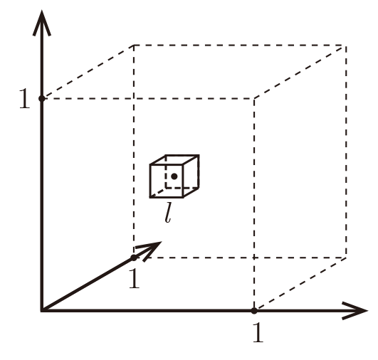
我们假设所有 training data 都在高维的某个 unit hypercube 中。假设 $d=10$, 对于某个 test point, 我们需要考虑离它最近的10个邻居。有了这10个邻居后，找到一个最小的能够包裹这10个邻居 hypercube，设它的边长为 $\ell$, 我们来看看这个 hypercube 的体积。

Formally, imagine the unit cube $[0,1]^d$. All training data is sampled uniformly within this cube, i.e. $\forall i, x_i\in[0,1]^d$, and we are considering the $k=10$ nearest neighbors of such a test point. Let $\ell$ be the edge length of the smallest hyper-cube that contains all $k$-nearest neighbor of a test point. Then $\ell^d\approx\frac{k}{n}$ and $\ell\approx\left(\frac{k}{n}\right)^{1/d}$. If $n= 1000$, how big is $\ell$?

So as $d\gg 0$ almost the entire space is needed to find the 10-NN. This breaks down the $k$-NN assumptions, because the $k$-NN are not particularly closer (and therefore more similar) than any other data points in the training set.

One might think that one rescue could be to increase the number of training samples, $n$, until the nearest neighbors are truly close to the test point. How many data points would we need such that $\ell$ becomes truly small? Fix $\ell=\frac{1}{10}=0.1$ $\Rightarrow$ $n=\frac{k}{\ell^d}=k\cdot 10^d$, which grows exponentially! For $d>100$ we would need far more data points than there are electrons in the universe...

Distances to hyperplanes¶

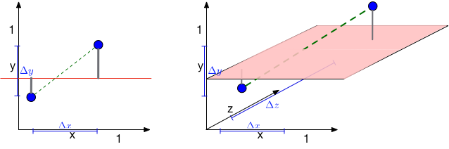
How about the distance to a hyperplane? Consider the following figure. There are two blue points and a red hyperplane. The following plot shows the scenario in 2d and the right plot in 3d. The distance to the red hyperplane remains unchanged as the third dimension is added. The reason is that the normal of the hyper-plane is orthogonal to the new dimension. This is a crucial observation.

**In $d$ dimensions, $d-1$ dimensions will be orthogonal to the normal of any given hyper-plane. 这$d-1$个维度对离hyperplane的距离毫无影响 **Movement in those dimensions cannot increase or decrease the distance to the hyperplane --- the points just shift around and remain at the same distance. As distances between pairwise points become very large in high dimensional spaces, distances to hyperplanes become comparatively tiny.

The curse of dimensionality has different effects on distances between two points and distances between points and hyperplanes.

An animation illustrating the effect on randomly sampled data points in 2D, as a 3rd dimension is added (with random coordinates). As the points expand along the 3rd dimension they spread out and their pairwise distances increase. However, their distance to the hyper-plane (z=0.5) remains unchanged --- so in relative terms the distance from the data points to the hyper-plane shrinks compared to their respective nearest neighbors.

Data with low dimensional structure¶

However, not all is lost. Data may lie in low dimensional subspace or on sub-manifolds. The true dimensionality of the data can be much lower than its ambient space. For example, an image of a face may require 18M pixels, a person may be able to describe this person with less than 50 attributes (e.g. male/female, blond/dark hair, …) along which faces vary.

An example of a data set in 3d that is drawn from an underlying 2-dimensional manifold. The blue points are confined to the pink surface area, which is embedded in a 3-dimensional ambient space.

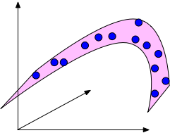
也就是说，前文提到的 curse of dimensionality 并不对实际模型应用起到太大印象，这是因为前面所讲的都是在随机的情况下，然而实际应用的可被预测的数据一般都具有一些隐含的结构（不然它怎么被预测呢）

k-NN summary¶

• $k$-NN is a simple and effective classifier if distances reliably reflect a semantically meaningful notion of the dissimilarity. (It becomes truly competitive through metric learning)
• As $n \to \infty$, $k$-NN becomes provably very accurate, but also very slow.
• As $d \gg 0$, points drawn from a probability distribution stop being similar to each other, and the $k$NN assumption breaks down.