K-means clustering

In unsupervised learning, we now only have features ($x_{1},\ldots,x_{n}$, where $x_{i} \in \mathbb{R}^{d}$) and no corresponding labels $y_{i}$. Therefore, we are not looking to make predictions. Instead, we are interested in uncovering structure in the feature vectors themselves.

In this lecture, we introduce K-means clustering. As we saw with KNN, sometimes we may suffer from the [curse of dimensionality](./2021-09-02-K-Nearest-Neighbors.md/#Curse of Dimenisionality), but any dataset that we can make predictions on must have “interesting” structures. K-Means will discover the clustered structure of the high dimensional data. (This is a bit different from PCA, which discovers low dimensional structure. PCA transforms high dimensional data points to be desribed by some fewer lower dimensional vectors. K-Means, on the other hand, describes a data point using its relation with each clusters: $x_i \to [c_1, c_2, \dots, c_k]$ where $c_i$ describes $x_i$’s relation with cluster $c_i$)

Objective¶

Given a set of $n$ data points $x_{1},\ldots,x_{n}$ with $x_{i} \in \mathbb{R}^{d}$, the goal of k-means clustering is to partition the data into $k$ groups where each group contains similar objects as defined by their Euclidean distances. Formally, we want to partition the n feature vectors into $k$ clusters $C_j$.

We now define what it means for a clustering to be “good.” We want to find clusters where the data points within each cluster are tightly grouped (i.e., exhibit low variability). Recall $\parallel x \parallel_{2}^{2} = x^{T}x$, so $\parallel x_{i} - x_{j} \parallel_{2}$ is the euclidean distance between the vectors $x_{i}$ and $x_{j}.$ Mathematically, for any cluster assignment we define

The smaller $Z$ is, the better we consider the clustering. Roughly speaking, we are trying to pick a clustering that minimizes the pairwise squared distances within each cluster (normalized by the cluster sizes).

The definition of $Z$ can be rewritten in terms of the centroid of each cluster: $$

\mu_{\ell} = \frac{1}{|\mathcal{C}{\ell}|}\sum\limits{i \in \mathcal{C}{\ell}}x{i}, Z_\ell = \sum\limits_{i \in \mathcal{C}{\ell}} \parallel x{i} - \mu_{\ell} \parallel_{2}^{2} $ \mu_{\ell}$is the mean/centroid of the points in cluster$ \ell$and$Z_\ell$ 为各 cluster 中所有点与其对应 centroid 的距离和

Now that we have a formal way to define a good clustering of points, we would like to solve

Unfortunately, solving this equation is not computationally feasible. We cannot do much better then simply trying all possible $k$ way partitions of the data and seeing which one yields the smallest objective value, so we have to relax our goal of finding the “best” clustering.

Lloyd’s algorithm for k-means¶

The practical approach we will take finding a good clustering is to use a local search algorithm.

• Local Search: 给一个现有的解决方案, interactively update it to a better and better clustering until it converges
• Converge: Do another local search, if our update result yields the same clusters we already have, we have a converge

This does not ensure convergence to the global solution.

Input: data $\{ x_{i}\}_{i = 1}^{n}$ and $k$

Initialize $C_{1},\ldots,C_{k}$

While not converged:

1. Compute $\mu_{\ell} = \frac{1}{|\mathcal{C}_{\ell}|}\sum\limits_{i \in \mathcal{C}_{\ell}}x_{i}$ for $\ell = 1,\ldots,k.$ [$O(dn)$ - 每个 feature vector 都对应一个 centroid]
2. Update $\mathcal{C}_{1},\ldots,\mathcal{C}_{k}$ by assigning each data point $x_{i}$ to the cluster whose centroid $\mu_{\ell}$ it is closest to. [$O(dnk)$ - 每个 feature vector 都要与 $k$ 个 centroid 算距离]
3. If the cluster assignments didn’t change, we have converged.

Return: cluster assignments $\mathcal{C}_{1},\ldots,\mathcal{C}_{k}$

This process actually has a nice feature that the objective function $Z$ is non-increasing (and only fails to decrease if the cluster assignments have converged). This is like loop invariant - termination.

The cost of Lloyd’s algorithm is $\mathcal{O}(ndk)$ per iteration. 注意每次计算（加法或乘法）花费的时间都与 dimension $d = |x_i|$ 有关。In practice its efficiency is strongly dependent on how many iterations it takes to converge.

How many clusters and how they are initialized¶

These 2 are the implicit input / super parameters we have to decide for a KNN algorithm.

Cluster Number $k$¶

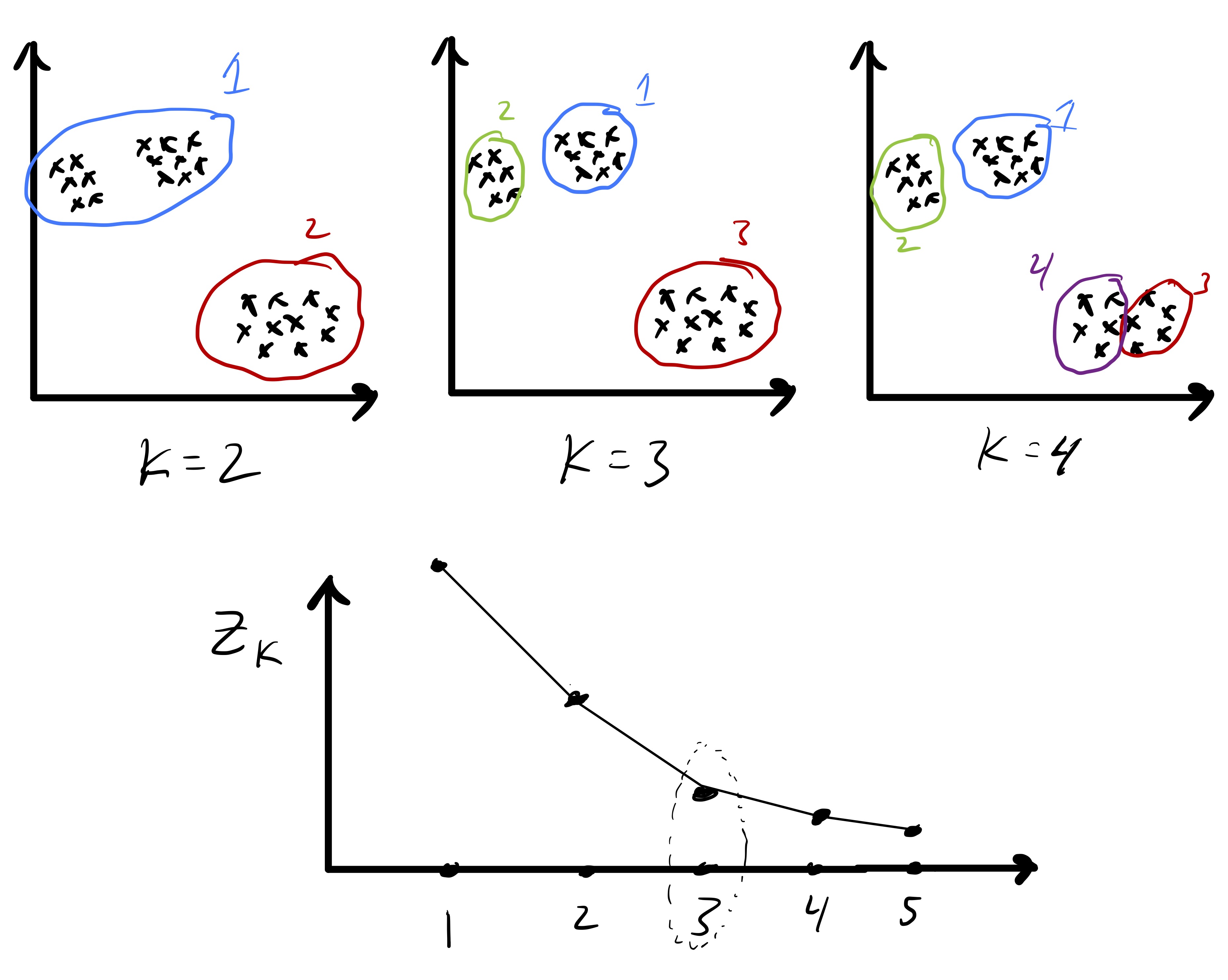
We want to pick a $k$ that minimizes $Z_k = Z(\mathcal{C}_{1},\ldots,\mathcal{C}_{k})$

However, this is problematic because we expect the in-cluster variation to decrease naturally with $k.$ In fact, if we have exactly $n$ clusters, $Z_{n} = 0$ since every point is its own cluster. So, instead, we often look for the point at which $Z_{k}$ stops decreasing quickly.

The intuition is that as $k\rightarrow k + 1$ if a single big cluster naturally subdivides into two clear clusters we will see that $Z_{k + 1} \ll Z_{k}$. In contrast, if we see $Z_{k + 1} \approx Z_{k}$, this might mean we have spitted up a clear cluster that does not naturally subdivide.

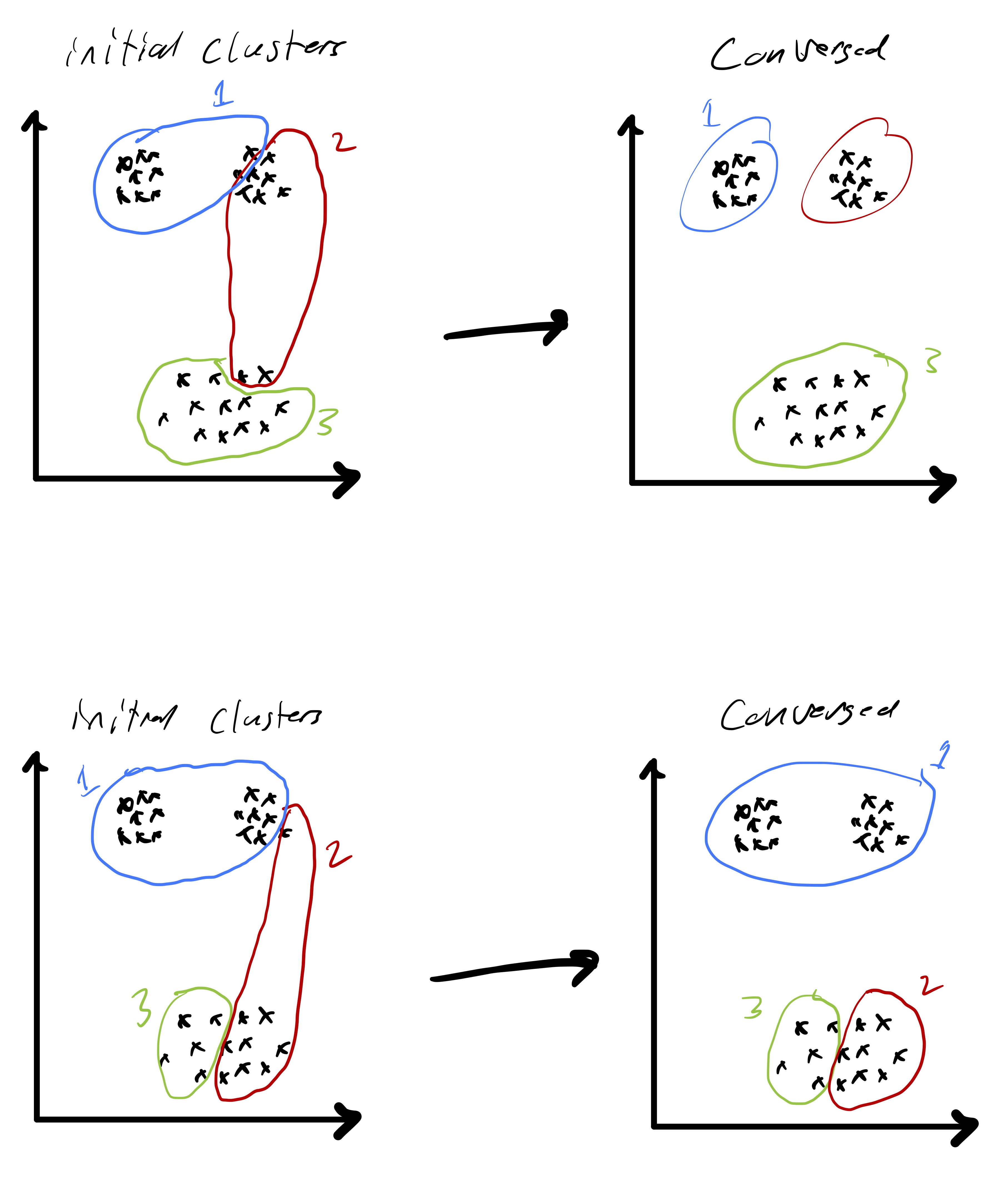
Initial Cluster Assignment¶

Initial cluster assignment This is particularly important because Lloyd’s algorithm only finds a local optima. So, very different initialization could result in convergence to very different solutions.

We can

• Choose several random clusterings and choose the one that gives the best result.
• Choose some random centroids, assign the rest points according to a weighted probability so that the farther they are from a centroid, the more likely they will be assigned to it. This is based on the idea that the cluster centers should be somewhat spread out.

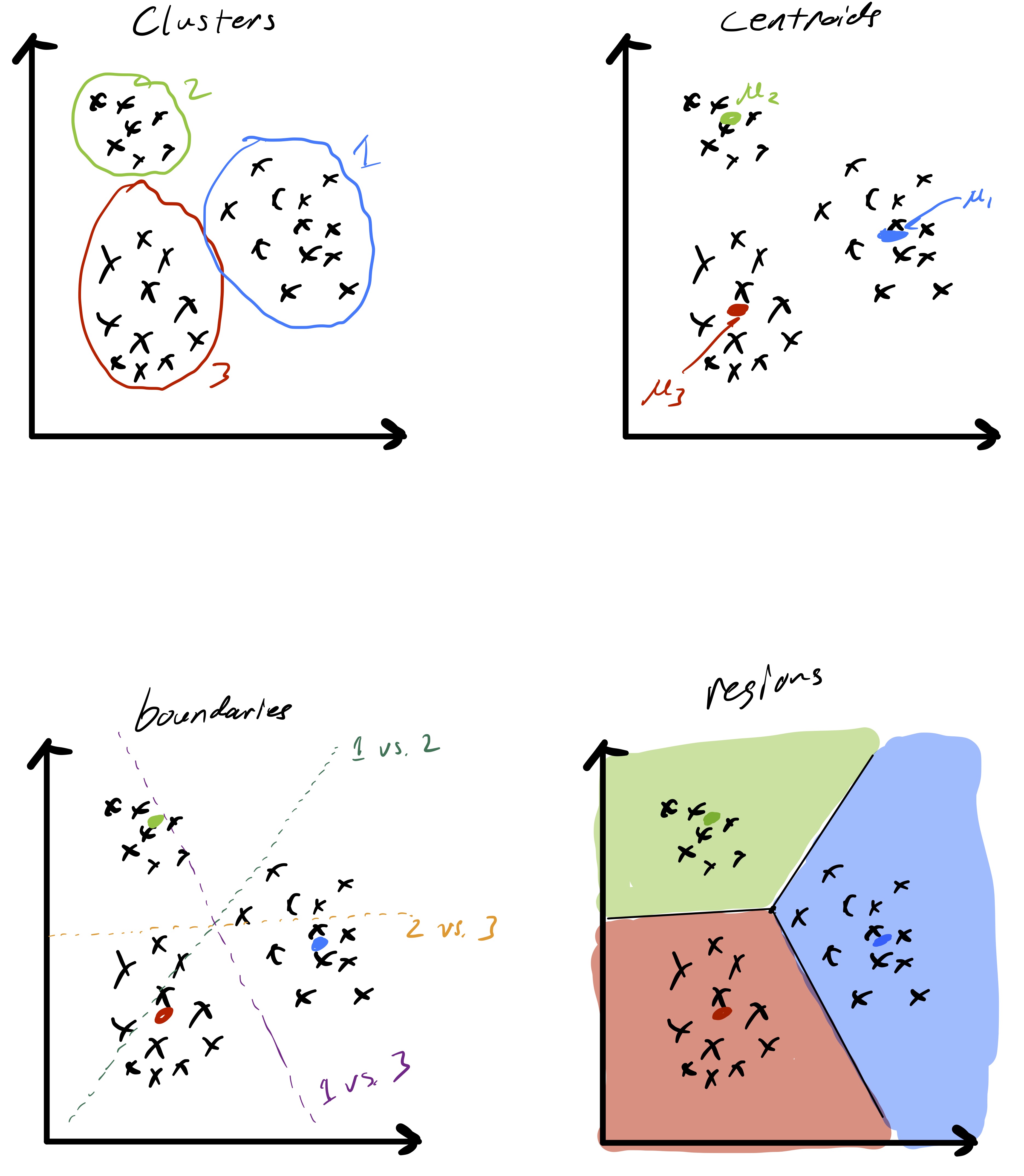
Decision boundaries¶

As said at the very beginning, unsupervised learning algorithm finds underlying structure of data points.

Observe that given two cluster centroids $\mu_{\ell}$ and $\mu_{\ell^{\prime}}$, the set of points equidistant from the two centroids defined as $\{ x \in \mathbb{R}^{d}\;|\; \parallel x - \mu_{\ell} \parallel_{2} = \parallel x - \mu_{\ell^{\prime}} \parallel_{2}\}$ is a line (就是 $\mu_{\ell}$ 和 $\mu_{\ell^{\prime}}$ 的中位线). This means that given a set of cluster centroids $\mu_{i},\ldots,\mu_{k}$ they implicitly partition space up into $k$ domains whose boundaries are linear.