The Perceptron

Assumptions¶

1. Binary classification (i.e. $y_i \in \{-1, +1\}$)
2. Data is linearly separable

Classifier¶

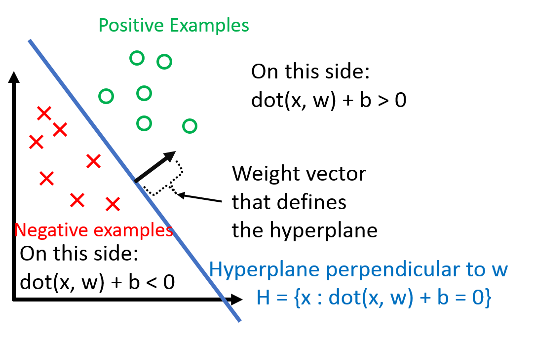
$w$ is the normal vector of the hyperplane. It defines this hyperplane. $b$ is the bias term (without the bias term, the hyperplane that $\mathbf{w}$ defines would always have to go through the origin). Dealing with $b$ can be a pain, so we ‘absorb’ it into the feature vector $\mathbf{w}$ by adding one additional constant dimension. Under this convention,

We can verify that

于是，我们通过把 b 藏在一个新的维度中“消除”了 b. Using this, we can simplify the above formulation of $h(\mathbf{x}_i)$ to

在这里我们看到两个例子，一个原数据在一维，一个原数据在二维。 (Left:) 我们无法找到一个过原点的平面将两个数据分开 (Right:) 但在我们再加入一维度时 ($x_i \to \begin{bmatrix} x_i \\1 \end{bmatrix}$)，就可以找到过原点的分隔平面了

Observation: Note that

where “classified correctly” means that $x_i$ is on the correct side of the hyperplane defined by $\mathbf{w}$. Also, note that the left side depends on $y_i \in {-1, +1}$ (it wouldn’t work if, for example $y_i \in {0, +1}$).

Perceptron Algorithm¶

An Intuitive Example¶

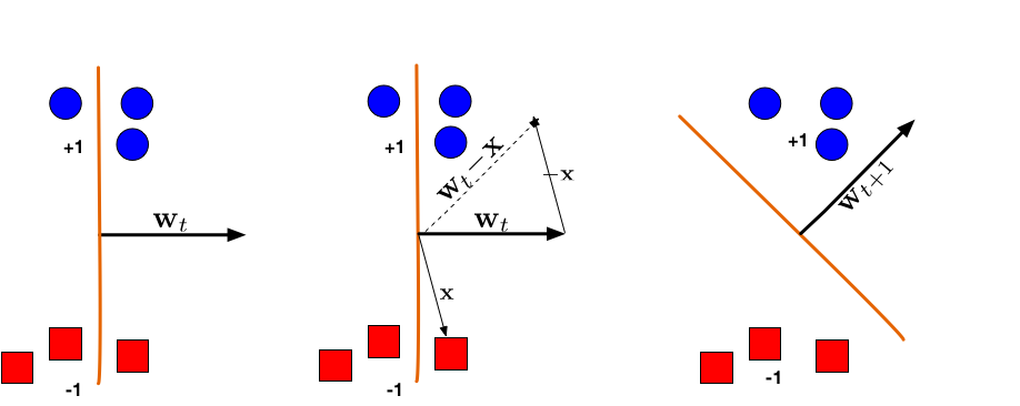
(Left:) The hyperplane defined by $\mathbf{w}_t$ misclassifies one red (-1) and one blue (+1) point. (Middle:) The red point $\mathbf{x}$ is chosen and used for an update. Because its label is -1 we need to subtract $\mathbf{x}$ from $\mathbf{w}_t$. (Right:) The udpated hyperplane $\mathbf{w}_{t+1}=\mathbf{w}_t-\mathbf{x}$ separates the two classes and the Perceptron algorithm has converged.

How did we update $w$?¶

Why do we want to update $w$ by setting $\vec{w} \prime = \vec{w} + y\vec{x}$?

Note we updated $w$ based on point $x$ because we classified $x$ incorrectly, so we want to move to a more correct direction. Let’s look at the classification result of $x$ after such an update: $\vec{w}\prime \cdot \vec{x}= (\vec{w} + y\vec{x}) \cdot \vec{x} = \vec{w} \cdot \vec{x} + y\vec{x}^2 \gt \vec{w} \cdot \vec{x}$. Though we still do not know whether $x$ is now labelled correctly ($\vec{w}\prime \cdot \vec{x}$), but at least we know the classification result is somewhat better because it increased a bit.

Proving Perceptron Converges¶

The Perceptron was arguably the first algorithm with a strong formal guarantee.

Claim¶

If a data set is linearly separable, the Perceptron will find a separating hyperplane in a finite number of updates. (If the data is not linearly separable, it will loop forever.)

Setup¶

The argument goes as follows: Suppose the answer classification hyperplane exists, so $\exists \mathbf{w}^*$ such that $\forall (\mathbf{x}_i, y_i) \in D, y_i(\mathbf{x}^\top \mathbf{w}^* ) > 0$.

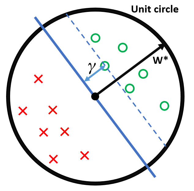
Now, suppose that we rescale each data point and the $\mathbf{w}^*$ such that all data points are within a unit hypersphere and $w^*$ normal vector of hyperplane is exactly on the unit sphere.

Let us define the Margin $\gamma$ of the hyperplane $\mathbf{w}^*$ as $\gamma = \min_{(\mathbf{x}_i, y_i) \in D}|\mathbf{x}_i^\top \mathbf{w}^*|$: 即所有数据点中离 hyperplane 最近的距离

Observe: $\forall\mathbf{x}, \text{we have } y(\mathbf{x}^\top \mathbf{w}^*)=|\mathbf{x}^\top \mathbf{w}^*|\geq \gamma$. Because $\mathbf{w}^*$ is a perfect classifier, so all training data points $(\mathbf{x},y)$ lie on the “correct” side of the hyper-plane and therefore $y=sign(\mathbf{x}^\top \mathbf{w}^*)$. The second inequality follows directly from the definition of the margin $\gamma$.

To summarize our setup:

• All inputs $\mathbf{x}_i$ live within the unit sphere
• There exists a separating hyperplane defined by $\mathbf{w}^*$, with $\|\mathbf{w}^*\|=1$ (i.e. $\mathbf{w}^*$ lies exactly on the unit sphere).
• $\gamma$ is the distance from this hyperplane (blue) to the closest data point.

WTS¶

If all of the above holds, then the Perceptron algorithm makes at most $1 / \gamma^2$ mistakes.

Strategy¶

Keeping what we defined above, consider the effect of an update ($\mathbf{w}$ becomes $\mathbf{w}+y\mathbf{x}$) on the two terms $\mathbf{w}^\top \mathbf{w}^*$ and $\mathbf{w}^\top \mathbf{w}$.

• $\mathbf{w} \cdot \mathbf{w}^*= \mathbf{w}^\top \mathbf{w}^*$: 我们希望它大，即我们的平面 $\mathbf{w}^\top$ 和正确答案平面 $\mathbf{w}^*$ 的方向越接近越好
• $\mathbf{w}\cdot\mathbf{w} = \mathbf{w}^\top \mathbf{w}$: 但同时，我们希望这个值小，因为我们不希望 $\mathbf{w}\cdot\mathbf{w}^*$ 大了是单纯因为 $\mathbf{w}$ 的大小变大了 ($\|\mathbf{w}^*\|=1$ 但谁都没规定 $\mathbf{w}$ 的大小)

Proof¶

We will use two facts:

• $y( \mathbf{x}^\top \mathbf{w})\leq 0$: This holds because $\mathbf x$ is misclassified by $\mathbf{w}$ - otherwise we wouldn’t make the update.
• $y( \mathbf{x}^\top \mathbf{w}^*) \ge \gamma \gt0$: First holds directly from definition of margin $\gamma$; second holds because $\mathbf{w}^*$ is a separating hyper-plane and classifies all points correctly.

Call the updated plane $\mathbf{w}\prime = \mathbf{w} + y\mathbf{x}$

1. Consider the effect of an update on $\mathbf{w}^\top \mathbf{w}^*$:

   $$\mathbf{w}\prime^\top \mathbf{w}^* = (\mathbf{w} + y\mathbf{x})^\top \mathbf{w}^*= \mathbf{w}^\top \mathbf{w}^* + y(\mathbf{x}^\top \mathbf{w}^*) \ge \mathbf{w}^\top \mathbf{w}^* + \gamma$$

   (7)

   The inequality follows from the fact that, for $\mathbf{w}^*$, the distance from the hyperplane defined by $\mathbf{w}^*$ to $\mathbf{x}$ must be at least $\gamma$ (i.e. $y (\mathbf{x}^\top \mathbf{w}^*)=|\mathbf{x}^\top \mathbf{w}^*|\geq \gamma$).

   his means that for each update, $\mathbf{w}^\top \mathbf{w}^*$ grows by at least $\gamma$.

2. Consider the effect of an update on $\mathbf{w}^\top \mathbf{w}$:

   $$\mathbf{w}\prime^\top \mathbf{w}\prime = (\mathbf{w} + y\mathbf{x})^\top (\mathbf{w} + y\mathbf{x}) = \mathbf{w}^\top \mathbf{w} + \underbrace{2y(\mathbf{w}^\top\mathbf{x})}_{<0} + \underbrace{y^2(\mathbf{x}^\top \mathbf{x})}_{0\leq \ \text{this value} \ \leq 1} \le \mathbf{w}^\top \mathbf{w} + 1$$

   (8)

   The inequality follows from the fact that

   • $2y(\mathbf{w}^\top \mathbf{x}) < 0$ as we had to make an update, meaning $\mathbf{x}$ was misclassified
   • $0\leq y^2(\mathbf{x}^\top \mathbf{x}) \le 1$ as $y^2 = 1$ and all $\mathbf{x}^\top \mathbf{x}\leq 1$ (because $\|\mathbf x\|\leq 1$).

   This means that for each update, $\mathbf{w}^\top \mathbf{w}$ grows by at most 1.

3. Now remember from the Perceptron algorithm that we initialize $\mathbf{w}=\mathbf{0}$. Hence, initially $\mathbf{w}^\top\mathbf{w}=0$ and $\mathbf{w}^\top\mathbf{w}^*=0$ and after $M$ updates the following two inequalities must hold:

   • $\mathbf{w}^\top\mathbf{w}^*\geq M\gamma$
   • $\mathbf{w}^\top \mathbf{w}\leq M$.

   We can then complete the proof:

   $$\begin{align} M\gamma &\le \mathbf{w}^\top \mathbf{w}^* &&\text{By (1)} \\ &=\|\mathbf{w}\|\cos(\theta) && \text{by definition of inner-product, where $\theta$ is the angle between $\mathbf{w}$ and $\mathbf{w}^*$.}\\ &\leq ||\mathbf{w}|| &&\text{by definition of $\cos$, we must have $\cos(\theta)\leq 1$.} \\ &= \sqrt{\mathbf{w}^\top \mathbf{w}} && \text{by definition of $\|\mathbf{w}\|$} \\ &\le \sqrt{M} &&\text{By (2)} \\ & \textrm{ }\\ &\Rightarrow M\gamma \le \sqrt{M} \\ &\Rightarrow M^2\gamma^2 \le M \\ &\Rightarrow M \le \frac{1}{\gamma^2} && \text{And hence, the number of updates $M$ is bounded from above by a constant.} \end{align}$$

   (9)

Problems and History¶

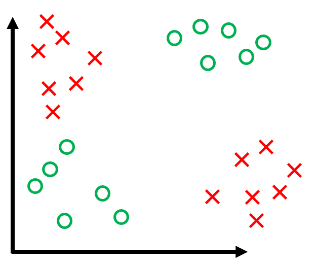
1. Perceptron suffers from the limitation of a linear model: If no separating hyperplane exists, perceptron will NEVER converge. (There will always be some points on the wrong side and it will iterate forever)

   

2. It does not generalize well either. Though it corrects all data points correctly, the decision boundary is almost arbitrary. And if a test point is given, Perceptron will very likely to classify it to the wrong side.

Especially suffered from the 1st problem, AI winter came as a result.