Gradient Descent

$argmin$ from Last Time¶

In the previous lecture on Logistic Regression we wrote down expressions for the parameters in our model as solutions to optimization problems that do not have closed form solutions. Specifically, given data $\{(x_{i},y_{i})\}_{i = 1}^{n}$ with $x_{i} \in \mathbb{R}^{d}$ and $y_{i} \in \{ + 1, - 1\}$ we saw that

and

These notes will discuss general strategies to solve these problems and, therefore, we abstract our problem to

where $\ell:\mathbb{R}^{d}\rightarrow\mathbb{R}.$ In other words, we would like to find the vector $w$ that makes $\ell(w)$ as small as possible.

Assumptions¶

Before diving into the mathematical and algorithmic details we will make some assumptions about our problem to simplify the discussion. Specifically, we will assume that:

1. $\ell$ is convex, so local minimum found is a global minimum.
2. $\ell$ is at least thrice continuously differentiable, so our Taylor approximations will work later.
3. There are no constraints placed on $w.$ It is common to consider the problem $\min\limits_{w \in \mathcal{C}}\ell(w)$ where $\mathcal{C}$ represents some constraints on $w$ (e.g., $w$ is entrywise non-negative). Adding constraints is a level of complexity we will not address here.

Defining Minimizer¶

We call $w^{\ast}$ a local minimizer of $\ell$ if:

$\exists \epsilon, s.t. \forall w \text{ where } \parallel w - w^{\ast} \parallel_{2} < \epsilon$ we have $\ell(w^{\ast}) \leq \ell(w).$

$w^*$ is a global minimizer if

$\forall w$, we have that $\ell(w^{\ast}) \leq \ell(w).$

Taylor Expansion¶

Recall that the first order Taylor expansion of $\ell$ centered at $w$ can be written as

where $g(w)$ is the gradient of $\ell$ evaluated at $w$, so $g(w) = \nabla\ell(w)$. This is the linear approximation of $\ell$ and has error $\mathcal{O}( \parallel p \parallel_{2}^{2})$.

Similarly, the second order Taylor expansion of $\ell$ centered at $w$ can be written as

where $H(w)$ is the Hessian of $\ell$ evaluated at $w$. This is the quadratic approximation of $\ell$ and has error $\mathcal{O}( \parallel p \parallel_{2}^{3})$.

Search Direction Methods¶

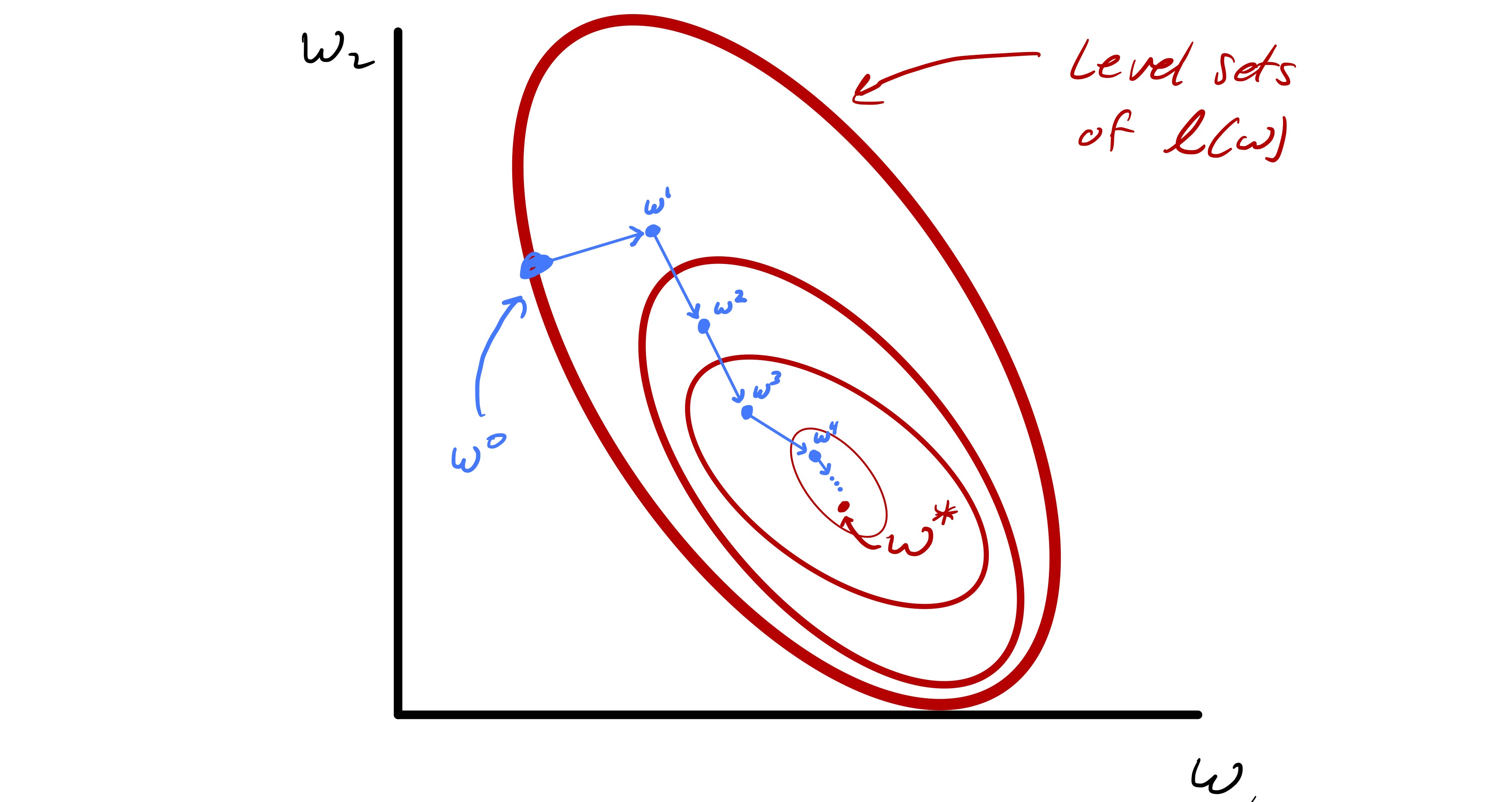
We can’t really find the exact point $w^*$ where a minimum is achieved. Therefore, the core idea to solve such problem is that given a starting point $w^{0}$ we construct a sequence of iterates $w^{1},w^{2},\ldots$ with the goal that $w^{k}\rightarrow w^{\ast}$ as $k\rightarrow\infty.$ In a search direction method we will think of constructing $w^{k + 1}$ from $w^{k}$ by writing it as $w^{k + 1} = w^{k} + s$ for some “step” $s.$ Concretely, this means our methods will have the following generic format:

Input: initial guess $w^{0}$

k = 0;

While not converged:

1. Pick a step $s$
2. $w^{k + 1} = w^{k} + s$ and $k = k + 1$
3. Check for convergence; if converged set $\hat{w} = w^{k}$

Return: $\hat{w}$

There are two clearly ambiguous steps in the above algorithm: how do we pick $s$ and how do we determine when we have converged. We will talk about two main methods used in picking $s$ and briefly touch on determining convergence.

Gradient Descent¶

We use the first order derivative to approximate our function $\ell$. At first attempt, we try to minimize this function. However, this is not attainable because linear function has no minimum - it just goes all the way to negative infinity. Therefore, we just take some step along this approximation to decrease the value by a bit.

If we directly look at the first order approximation, gradient descent can be also interpreted as follows: given we are currently at $w^{k},$ determine the direction in which the function decreases the fastest (along the gradient) at this point and update our $w$ by taking a step in that direction. Consider the linear approximation to $\ell$ at $w^{k}$ provided above by the Taylor series:

then the fastest direction to descend is simply $s = - \nabla\ell(w^{k})$, so we just go along the gradient. We want to get a smaller value so go along the negative direction. We go some $\alpha \gt 0$ distance, so set $s$ as

$\alpha$¶

$\alpha$ is often referred to as the step size in classical optimization, but learning rate in Machine Learning.

1. line search - find the best $\alpha$, but expensive so we don’t use it
2. fix $\alpha$ - might not converge
3. decay $\alpha$ - set $\alpha = c/k$ at iteration $k$ for any constant $c > 0$, so we take big step early on and take smaller steps as we think we are going to the minimizer. This guarantees convergence.

Adagrad¶

Adagrad (technically, diagonal Adagrad) can be seen as an improvement of decay $\alpha$, where we determine the step size on an entry basis by the steepness of the function - big “decay” for steep direction, and small “decay” for flat direction.

Note in gradient descent, we have the same learning rate across entries, which basically says “we learn the same amount for both rare and common features”. However, we want to have

• rare features - large learning rate. If set the learning rate too small, we won’t be able to change these rarely changed values at all; As we update the model, we always have a small gradient along the rare features, because these rarely occurred events usually have a subtle effect on the model (whether have a pet, whether they follow the traffic light, ...) If we draw a graph of our function, it is flat at this direction.
• common features - low learning rate. If set the learning rate too large, our model will simply jump back and forth because of these common features; As we update the model, we always have a large running gradient along the common features , because they usually have the greatest influence on model (Gender, Race, Age). If we draw a graph of our function, it is steep at this direction.

Therefore, we decrease the step size by a lot along the direction where we already took a large step (that’s along the steep direction, common features) and decrease the step size only by a bit along the direction where we just took a small step (the flat direction, rare features.)

Adagrad keeps track of history of steepness by keeping a running average of the squared gradient at each entry. It then sets a small learning rate for variables with large past gradients and a large learning rate for features with small past gradients.

Input: $\ell,$ $\nabla\ell,$ parameter $\epsilon > 0,$ and initial learning rate $\alpha.$

Set $w_{j}^{0} = 0$ and $z_{j} = 0$ for $j = 1,\ldots,d.$ k = 0;

While not converged:

1. Compute the gradient $\nabla w^k$ and record values for each entry of the gradient $g_{j} = [\nabla w^k]_j$
2. For each dimension $j$, calculate the moving sum of squared gradient at dimension $j$: $z_{j} = z_{j} + g_{j}^{2}$ for $j = 1,\ldots,d$
3. $w_{j}^{k + 1} = w_{j}^{k} - \alpha\frac{g_{j}}{\sqrt{z_{j} + \epsilon}}$ for $j = 1,\ldots,d.$
4. $k = k + 1$
5. Check for convergence; if converged set $\hat{w} = w^{k}$

Return: $\hat{w}$

Convergence¶

Assuming the gradient is non-zero, we can show that there is always some small enough $\alpha$ such that $\ell(w^{k} - \alpha \nabla\ell(w^{k})) < \ell(w^{k}).$ In particular, we have

Since $(\nabla\ell(w^{k}))^{T}\nabla\ell(w^{k}) > 0$ and $\alpha^{2}\rightarrow 0$ faster than $\alpha$ as $\alpha\rightarrow 0$, we conclude that for some sufficiently small $\alpha > 0$ we have that $\ell(w^{k} - \alpha \nabla\ell(w^{k})) < \ell(w^{k}).$

Newton’s Method¶

Newton’s Method instead uses the second order derivative to approximate $\ell$. We will pretend our approximation represents $\ell$ very well, finds the minimum point of our quadratic approximation, and claim it also to be the minimum of our original function $\ell$. This works really well when our function indeed looks similar to a quadratic function locally, but when our approximation is off, the result will be way off and may never converge.

Specifically, we now chose a step by explicitly minimizing the quadratic approximation to $\ell$ at $w^{k}$. We can find this minimum because $\ell$ is convex. To accomplish this, we solve

by differentiating and setting the gradient equal to zero. Since the gradient of our quadratic approximation is $\nabla\ell(w^{k}) + H(w^{k})s$ this implies that $s$ solves the linear system

This system is solvable because convex $\ell$ guarantees a positive semi-definite $H(w)$ for all $w$. (In fact, we need to solve this function by having a positive definite $H$, which is guaranteed by a strictly convex $\ell$, but we will introduce a workaround later)

Potential Issues¶

Bad Approximation¶

Newton’s method has very good properties in the neighborhood of a strict local minimizer and once close enough to a solution it converges rapidly. However, if you are far from where the quadratic approximation is valid, Newton’s Method can diverge or enter a cycle. Practically, a fix for this is to introduce a step size $\alpha > 0$ and formally set

We typically start with $\alpha = 1$ since that is the proper step to take if the quadratic is a good approximation. However, if this step seems poor (e.g. $\ell(w^{k} + \alpha s) > \ell(w^{k})$) then we can decrease $\alpha$ at that iteration.

Positive Semi-Definite $H(w^k)$¶

• When $\ell$ is convex but not strictly convex we can only assume that $H(w^{k})$ is positive semi-definite
• When the original function / our approximation is really flat (remember Hessian matrix represents curvature), so $H$ is not invertible.

In principle this means that $H(w^{k})s = - \nabla\ell(w^{k})$ may not have a solution. Or, if $H(w^{k})$ has a zero eigenvalue then we always have infinite solutions. A “quick fix” is to simply solve

for some small parameter $\epsilon$ instead. This lightly regularizes the quadratic approximation to $\ell$ at $w^{k}$ and ensures it has a strict global minimizer.

Slow Running Time¶

Newton’s method requires a second order approximation of the original function, which involved the Hessian matrix $H$. There are a lot of parameters to compute compared to a first order approximation.

Checking for convergence¶

1. Relative change in the iterates, i.e. $\frac{\parallel w^{k + 1} - w^{k} \parallel_{2}}{\parallel w^{k} \parallel_{2}} < \delta_{1}$ for some small $\delta_{1} > 0$.
2. A reasonably small gradient, i.e., $\parallel \nabla\ell(w^{k}) \parallel_{2} < \delta_{2}$ for some small $\delta_{2} > 0$.