When you have a bunch of Random Variables adding together, it is likely to be Gaussian distributed, but we do want these Random Variables to have finite mean and finite variance. In this case, they will be Gaussian according to the Central Limit Theorem.
The sum of a bunch finite mean but infinite variance Random Variables doesn’t usually converge, but when it does, it gives Power Law Distribution. Examples of power law: wealth per person, word frequency.
Power Law is scale free: Select an arbitrary part of the graph and zoom into it, we will find it have the exact same shape as the original graph.
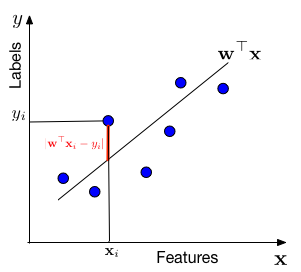
where ϵ is a the noise: we said label is “somewhat” linear, so they can’t always be exactly on the line. The ϵ here is the offset between the label and the line.
We also assume that the noise is Gaussian distributed
so for a fixed distance, each point has the same probability of being that distance away from the line. It is also reasonable to have mean as 0, because if it >0, it means majority points a more off to the above, so we can just move our line up a bit; similar for <0, we just move the line down a bit.
根据我们这里的假设,可以通过将 ϵi 的 distribution 向我们的模型预测直线 w⊤xi 移动得到
w=wargmaxP(y1,x1,...,yn,xn∣w)=wargmaxi=1∏nP(yi,xi∣w)=wargmaxi=1∏nP(yi∣xi,w)P(xi∣w)=wargmaxi=1∏nP(yi∣xi,w)P(xi)=wargmaxi=1∏nP(yi∣xi,w)=wargmaxi=1∑nlog[P(yi∣xi,w)]=wargmaxi=1∑n[log(2πσ21)+log(e−2σ2(xi⊤w−yi)2)]=wargmax−2σ21i=1∑n(xi⊤w−yi)2=wargminn1i=1∑n(xi⊤w−yi)2Because data points are independently sampled.Chain rule of probability.xi is independent of w, we only model P(yi∣x)P(xi) is a constant - can be droppedlog is a monotonic functionPlugging in probability distributionFirst term is a constant, and log(ez)=zn1 makes the loss interpretable (average squared error).
Therefore, maximizing parameter w is equivalent to minimizing a loss function, l(w)=n1∑i=1n(xi⊤w−yi)2. This particular loss function is also known as the squared loss or Ordinary Least Squares (OLS). OLS has a closed form:
w=(XX⊤)−1Xy⊤ where X=[x1,…,xn] and y=[y1,…,yn].
With MAP, we can have a prior belief on our w, so we make the additional assumption:
P(w)∼N(0,τ2I)=2πτ21e−2τ2w⊤w This is to say: all features have a same deviation τ2 and are drawn independently from each other, so each feature has the same probability of being big or small.