SVM - Support Vector Machine

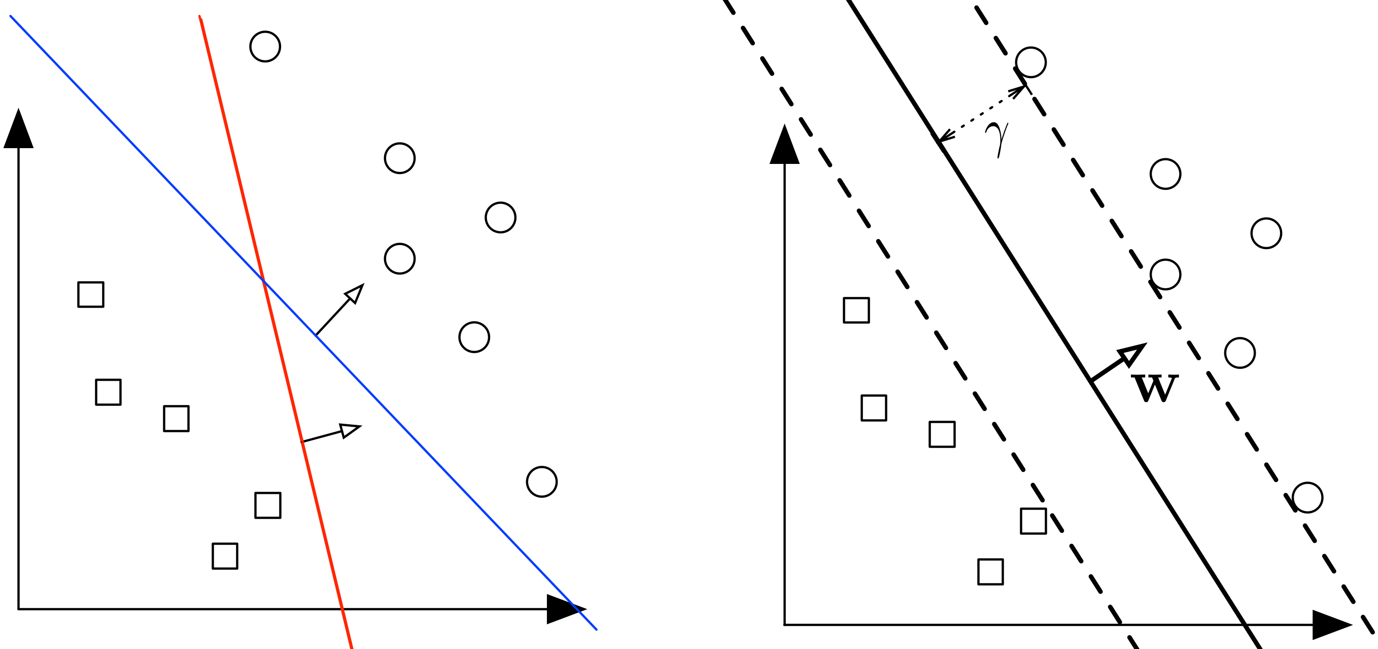
The left picture is what we have achieved so far with a perceptron. The perceptron can give us either the blue line or a red line, so the result does not generalize well. We can view SVM (on the right) as an improvement of the Perceptron - it finds the one that maximizes the distance to the closest data points from both classes. We say it is the maximum margin separating hyperplane.

Defining Margin¶

We know the distance from a point $\textbf x$ to a plane $\mathcal{H} = \left\{\mathbf{x}\vert{}\mathbf{w}^T\mathbf{x}+b=0\right\}$ is $\mathbf{d(x_i, \mathcal H)} = \frac{\left | \mathbf{w}^T\mathbf{x}+b \right |}{\left \| \mathbf{w} \right \|_{2}}$.

Using the definition of margin from Perceptron, we have margin of $\mathcal{H}$ with respect to out dataset $D$ is $\gamma(\mathbf{w},b)=\min_{\mathbf{x}\in D}\frac{\left | \mathbf{w}^T\mathbf{x}+b \right |}{\left \| \mathbf{w} \right \|_{2}}$

By definition, the margin and hyperplane are scale invariant: $\gamma(\beta\mathbf{w},\beta b)=\gamma(\mathbf{w},b), \forall \beta \neq 0$

Max Margin Classifier¶

We can formulate our search for the maximum margin separating hyperplane as a constrained optimization problem. The objective is to maximize the margin under the constraints that all data points must lie on the correct side of the hyperplane:

If we plug in the definition of $\gamma$ we obtain:

Maximizing minimum seems almost impossible to do, so we want to remove the $min$ in the value we are trying to maximize. We can move this $min$ to be a new constraint: Because the hyperplane is scale invariant, we can fix the scale of $\mathbf{w},b$ anyway we want. We choose them such that

so our objective becomes:

Add our re-scaling as an equality constraint to the overall problem, our new optimization problem to solve is:

These two new constraints are equivalent to $\forall i \ y_{i}(\mathbf{w}^T \mathbf{x}_{i}+b) \geq 1$ (Don’t ask me how to do a right to left proof, I do not know), so we can rewrite our optimization problem as:

This new formulation is simply a quadratic optimization problem. The objective is quadratic and the constraints are all linear. We can be solve it efficiently with any QCQP (Quadratically Constrained Quadratic Program) solver. It has a unique solution whenever a separating hyper plane exists. It also has a nice interpretation: Find the simplest hyperplane (where simpler means smaller $\mathbf{w}^\top\mathbf{w}$) such that all inputs lie at least 1 unit away from the hyperplane on the correct side.

An intuition behind this formula is: the new constraint can be written as $|\mathbf{w}^T \mathbf{x}_{i}+b| \geq 1$. Note this is $| \mathbf{w}|_{2} \; \mathbf{d(x_i, \mathcal H)} \geq 1$, so $\sqrt{\mathbf{w}^T\mathbf{w}} \; \mathbf{d(x_i, \mathcal H)} \geq 1$. Since we are minimizing $\sqrt{\mathbf{w}^T\mathbf{w}}$, the only way we can achieve the greater than 1 constraint is to make $\mathbf d$ big. This is exactly what we want.

We can write the prediction result as $h({\mathbf{x}_i}) = w^{\top}{\mathbf{x}_i}+b$, so $h(\mathbf{x}_i)y_{i}$ represents classification result correctness. If it is positive, the prediction is correct. And the bigger this value, the more correct we get. If it is negative, the prediction is wrong.

Support Vectors¶

For the optimal $\mathbf{w},b$ pair, some training points will have tight constraints, i.e.

We refer to these training points as support vectors. These vectors define the maximum margin of the hyperplane to the data set and they therefore determine the shape of the hyperplane. If you were to move one of them and retrain the SVM, the resulting hyperplane would change. The opposite is the case for non-support vectors.

SVM with soft constraints¶

If the data is low dimensional it is often the case that there is no separating hyperplane between the two classes, so there is no solution to the optimization problems above. We can fix this by allowing the constraints to be violated (distance of $x_i$ to the hyperplane to be greater than the margin) ever so slight with the introduction of slack variables $\xi$. At the same time, we don’t want to loose the constraints too much, so we also minimize these slack variables along the way.

As the slack $\xi_i$ gets larger, we allow point $x_i$ to be closer to the hyperplane $\ y_{i}(\mathbf{w}^T\mathbf{x}_{i}+b) \lt 1$, or even on the other side $\ y_{i}(\mathbf{w}^T\mathbf{x}_{i}+b) \lt 0$

If C is very large, the SVM becomes very strict and tries to get all points to be on the right side of the hyperplane. If C is very small, the SVM becomes very loose and may “sacrifice” some points to obtain a simpler (i.e. lower $\|\mathbf{w}\|_2^2$) solution.

Unconstrained Formulation¶

We will express our “SVM with soft constraints” in an unconstrained form.

Note if $y_{i}(\mathbf{w}^T \mathbf{x}_{i}+b)<1$, so current point is too close (or on the other side) to the plane, $\xi_i$ is the distance away from the margin point. If point $x_i$ is just as far as other good points, $\xi_i$ is simply 0. Formulate this in the equation below:

which is equivalent to the following closed form:

This closed form is called the hinge loss. If we plug this closed form into the objective of our SVM optimization problem, we obtain the following unconstrained version as loss function and regularizer:

We optimize SVM paramters $\mathbf{w},b$ by minimizing this loss function just like we did in logistic regression (e.g. through gradient descent). The only difference is that we have the hinge loss here instead of the logistic loss.