Empirical Risk Minimization - Incomplete CS Notes @ Cornell

Recap¶

Remember the unconstrained SVM Formulation

\min_{\mathbf{w}}\ C\underset{Hinge-Loss}{\underbrace{\sum_{i=1}^{n}\max[1-y_{i}\underset{h({\mathbf{x}_i})}{\underbrace{(w^{\top}{\mathbf{x}_i}+b)}},0]}}+\underset{l_{2}-Regularizer}{\underbrace{\left\Vert w\right\Vert _{z}^{2}}}

(1)

where $h({\mathbf{x}_i}) = w^{\top}{\mathbf{x}_i}+b$ is our prediction, the hinge loss is the SVM’s error function, and the $\left.l_{2}\right.$ -regularizer reflects the complexity of the solution, and penalizes complex solutions (those with big $w$ ).

We can generalize problem of this form as empirical risk minimization with

loss function $\ell$ : continuous function which penalizes training error
regularizer $r$ : shape your model to the shape your prefer (usually a continuous function which penalizes classifier complexity)

\min_{\mathbf{w}}\frac{1}{n}\sum_{i=1}^{n}\underset{Loss}{\underbrace{l(h_{\mathbf{w}}({\mathbf{x}_i}),y_{i})}}+\underset{Regularizer}{\underbrace{\lambda r(w)}},

(2)

In SVM, $\ell = \max[1-y_{i}h({\mathbf{x}_i}), 0]$ , $r(w) = \left\Vert w\right\Vert _{z}^{2}$ , $\lambda = \frac{1}{C}$ .

Binary Classification Loss Functions¶

Loss function in binary classification problem is always about $h(\mathbf{x}_i)y_{i}$ - classification result correctness.

Loss $\ell$	Usage	Comments
Hinge-Loss $\max\left[1-h_{\mathbf{w}}(\mathbf{x}_{i})y_{i},0\right]^{p}$	Standard SVM( $\left.p=1\right.$ ) Differentiable/Squared Hinge Loss SVM ( $\left.p=2\right.$ )	When used for Standard SVM, the loss function denotes the size of the margin between linear separator and its closest points in either class. Only differentiable everywhere with $\left.p=2\right.$ , but then it penalizes mistake much more aggressively.
Log-Loss $\left.\log(1+e^{-h_{\mathbf{w}}(\mathbf{x}_{i})y_{i}})\right.$	Logistic Regression	Very popular loss functions in ML, since its outputs are well-calibrated probabilities.
Exponential Loss $\left. e^{-h_{\mathbf{w}}(\mathbf{x}_{i})y_{i}}\right.$	AdaBoost	This function is very aggressive. The loss of a mis-prediction increases exponentially with the value of $-h_{\mathbf{w}}(\mathbf{x}_i)y_i$ . This can lead to nice convergence results, for example in the case of Adaboost, but it can also cause problems with noisy data or when you simply mistakenly mislabeled data.
Zero-One Loss $\left.\delta(\textrm{sign}(h_{\mathbf{w}}(\mathbf{x}_{i}))\neq y_{i})\right.$	Actual Classification Loss	Non-continuous and thus impractical to optimize.

Figure 4.1: Plots of Common Classification Loss Functions:
x-axis: $\left.h(\mathbf{x}_{i})y_{i}\right.$ , or “correctness” of prediction
y-axis: loss value

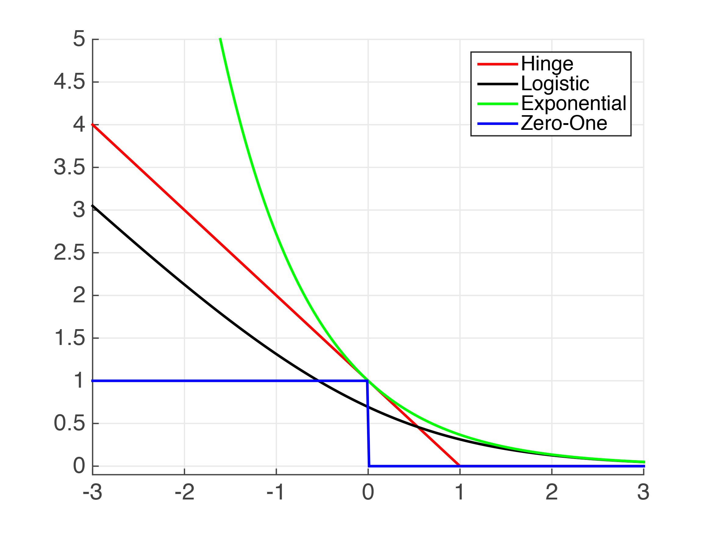
A minor point: from the graph we know that Exponential Loss is a strict upperbound of 0/1 Loss. This will be useful later for proving its convergence.

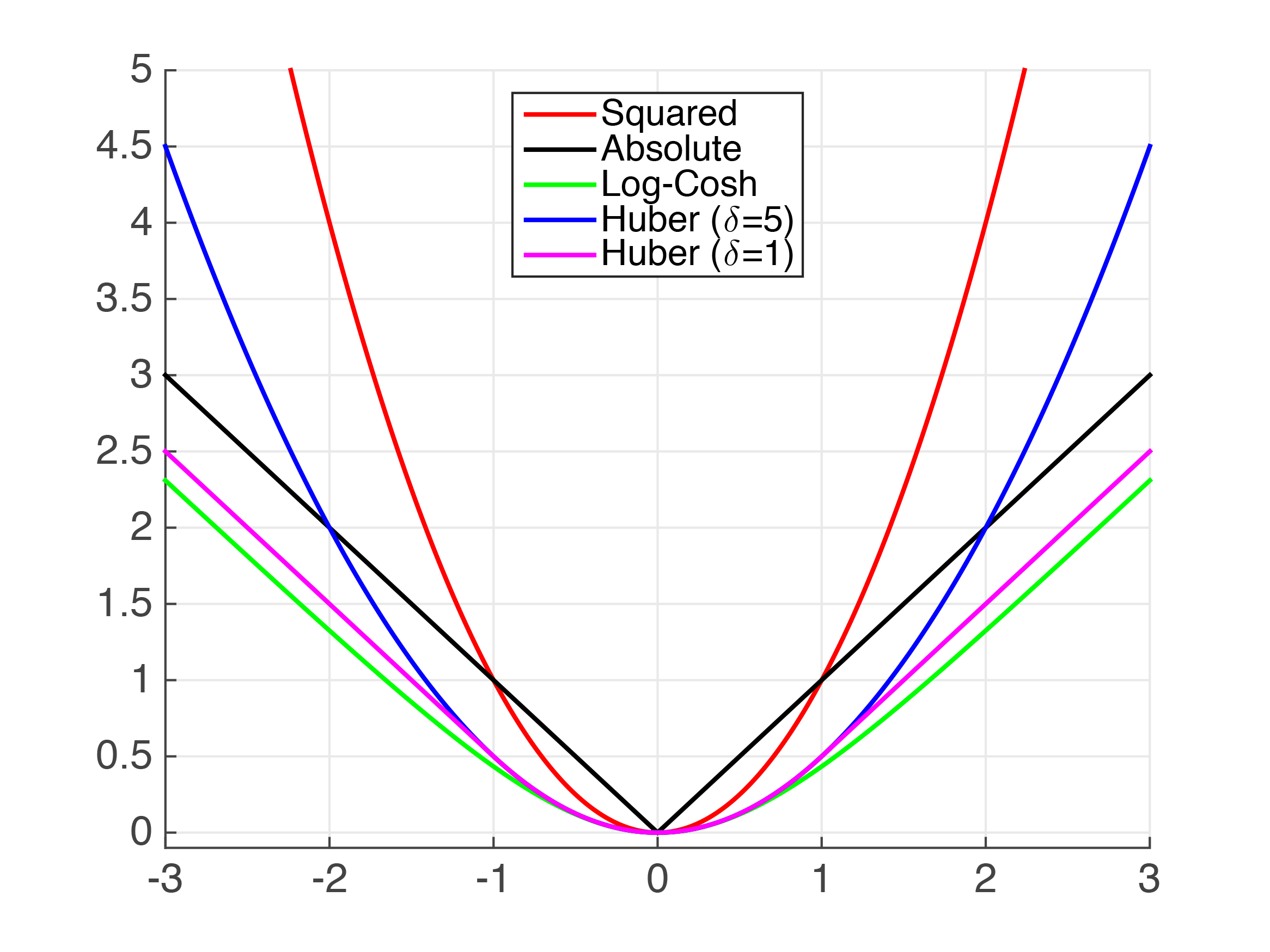
Regression Loss Functions¶

Loss function in regression is always about the offset between prediction and original value $z = y - h(\mathbf x)$ .

Loss $\ell$	Comments
Squared Loss $\left(h(\mathbf{x}_{i})-y_{i}\right)^{2}$	Most popular regression loss function Also known as Ordinary Least Squares (OLS) ADVANTAGE: Differentiable everywhere DISADVANTAGE: Somewhat sensitive to outliers/noise Estimates Mean Label
Absolute Loss $\left\|h(\mathbf{x}_{i})-y_{i}\right\|$	Also a very popular loss function Estimates Median Label ADVANTAGE: Less sensitive to noise DISADVANTAGE: Not differentiable at 0 (the point which minimization is intended to bring us to)
Huber Loss $\begin{cases} \frac{1}{2}\left(h(\mathbf{x}_{i})-y_{i}\right)^{2} & \text{if} \left\|h(\mathbf{x}_{i})-y_{i}\right\|<\delta\\ \delta(\left\|h(\mathbf{x}_{i})-y_{i}\right\|-\frac{\delta}{2})& \text{otherwise} \end{cases}$	Also known as Smooth Absolute Loss ADVANTAGE: “Best of Both Worlds” of Squared and Absolute Loss Once-differentiable Takes on behavior of Squared-Loss when loss is small, and Absolute Loss when loss is large.
Log-Cosh Loss $\left.log(cosh(h(\mathbf{x}_{i})-y_{i}))\right. ,\left.cosh(x)=\frac{e^{x}+e^{-x}}{2}\right.$	ADVANTAGE: Similar to Huber Loss, but twice differentiable everywhere

In the squared loss, the biggest loss shadows all the other losses - it wants to use whatever’s possible to decrease the biggest loss. We say the absolute loss is somewhat an “improvement” of the squared loss because it treats all losses more fairly. For example, in squared loss, 10 samples each diff by 1 is 10 loss, but 1 sample differs by 10 is 100 loss. On the other hand, 10 diff by 1 and 1 diff by 10 are both 10 loss in absolute value loss.

Figure 4.2: Plots of Common Regression Loss Functions:
x-axis: $h(\mathbf{x}_{i})-y_{i}$ , or “error” of prediction
y-axis: loss value

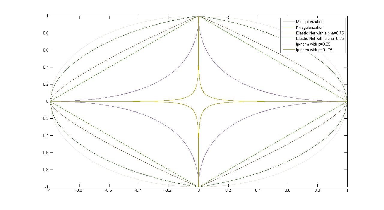
Regularizers¶

Remember with Lagrange multipliers, which says for all $B\geq0$ , there exists $\lambda\geq0$ such that the two problems below are equivalent, and vice versa.

\min_{\mathbf{w}} f(\mathbf w) \textrm { s.t. } g(\mathbf{w})\leq B \Leftrightarrow \min_{\mathbf{w}} f(\mathbf w) +\lambda g(\mathbf{w})

(3)

We can therefore change the formulation of the optimization problem with regularizers to obtain a better geometric intuition:

\min_{\mathbf{w},b} \sum_{i=1}^n\ell(h_\mathbf{w}(\mathbf{x}),y_i)+\lambda r(\mathbf{w}) \Leftrightarrow \min_{\mathbf{w},b} \sum_{i=1}^n\ell(h_\mathbf{w}(\mathbf{x}),y_i) \textrm { subject to: } r(\mathbf{w})\leq B

(4)

Regularizer $r(\mathbf{w})$	Properties
$l_{2}$ -Regularization $\left.r(\mathbf{w}) = \mathbf{w}^{\top}\mathbf{w} = \|{\mathbf{w}}\|_{2}^{2}\right.$	ADVANTAGE: Strictly Convex, Differentiable DISADVANTAGE: Dense Solutions (it uses weights on all features, i.e. relies on all features to some degree. Ideally we would like to avoid this)
$l_{1}$ -Regularization $\left.r(\mathbf{w}) = \|\mathbf{w}\|_{1}\right.$	Convex (but not strictly) DISADVANTAGE: Not differentiable at 0 (the point which minimization is intended to bring us to) Effect: Sparse (i.e. not Dense) Solutions
$l_p$ -Norm $\left.\|{\mathbf{w}}\|_{p} = (\sum\limits_{i=1}^d v_{i}^{p})^{1/p}\right.$	(often $\left.0<p\leq1\right.$ ) DISADVANTAGE: Non-convex, Not differentiable, Initialization dependent ADVANTAGE: Very sparse solutions

Figure 4.3: Plots of Common Regularizers

Famous Special Cases¶

This section includes several special cases that deal with risk minimization, such as Ordinary Least Squares, Ridge Regression, Lasso, and Logistic Regression. Table 4.4 provides information on their loss functions, regularizers, as well as solutions.

Loss and Regularizer	Comments
Ordinary Least Squares $\min_{\mathbf{w}} \frac{1}{n}\sum\limits_{i=1}^n (\mathbf{w}^{\top}x_{i}-y_{i})^{2}$	Squared Loss No Regularization Closed form solution: $\left.\mathbf{w}=(\mathbf{X}\mathbf{X}^\top)^{-1}\mathbf{X}\mathbf{y}^{\top}\right.$ $\left.\mathbf{X}=[\mathbf{x}_{1}, ..., \mathbf{x}_{n}]\right.$ $\left.\mathbf{y}=[y_{1},...,y_{n}]\right.$
Ridge Regression $\min_{\mathbf{w}} \frac{1}{n}\sum\limits_{i=1}^n (\mathbf{w}^{\top}x_{i}-y_{i})^{2}+\lambda\|{w}\|_{2}^{2}$	Squared Loss $l_{2}$ -Regularization $\left.\mathbf{w}=(\mathbf{X}\mathbf{X}^{\top}+\lambda\mathbb{I})^{-1}\mathbf{X}\mathbf{y}^{\top}\right.$
Lasso $\min_{\mathbf{w}} \frac{1}{n}\sum\limits_{i=1}^n (\mathbf{w}^{\top}\mathbf{x}_{i}-{y}_{i})^{2}+\lambda\|\mathbf{w}\|_{1}$	+ sparsity inducing (good for feature selection) + Convex - Not strictly convex (no unique solution) - Not differentiable (at 0) Solve with (sub)-gradient descent or SVEN
Elastic Net $\min_{\mathbf{w}} \frac{1}{n}\sum\limits_{i=1}^n (\mathbf{w}^{\top}\mathbf{x}_{i}-{y}_{i})^{2}+\left.\alpha\|\mathbf{w}\|_{1}+(1-\alpha)\|{\mathbf{w}}\|_{2}^{2}\right.$ $\left.\alpha\in[0, 1)\right.$	ADVANTAGE: Strictly convex (i.e. unique solution) + sparsity inducing (good for feature selection) + Dual of squared-loss SVM, see SVEN DISADVANTAGE: - Non-differentiable
Logistic Regression $\min_{\mathbf{w},b} \frac{1}{n}\sum\limits_{i=1}^n \log{(1+e^{-y_i(\mathbf{w}^{\top}\mathbf{x}_{i}+b)})}$	Often $l_{1}$ or $l_{2}$ Regularized Solve with gradient descent. $\left.\Pr{(y
Linear Support Vector Machine $\min_{\mathbf{w},b} C\sum\limits_{i=1}^n \max[1-y_{i}(\mathbf{w}^\top{\mathbf{x}_i+b}), 0]+\|\mathbf{w}\|_2^2$	Typically $l_2$ regularized (sometimes $l_1$ ). Quadratic program. When kernelized leads to sparse solutions. Kernelized version can be solved very efficiently with specialized algorithms (e.g. SMO)

Table 4.4: Special Cases

CS4780 Intro to Machine Learning

SVM - Support Vector Machine

CS4780 Intro to Machine Learning

Midterm Review