Bias-Variance Tradeoff
Setting Up
As usual, we are given a training dataset , drawn i.i.d. from some distribution . Throughout this lecture we assume a regression setting, i.e. . In this lecture we will decompose the generalization error of a classifier into three rather interpretable terms.
Expected Label
Even though we have the same features , their labels can be different . For example, if your vector describes features of house (e.g. #bedrooms, square footage, ...) and the label its price, you could imagine two houses with identical description selling for different prices. So for any given feature vector , there is a distribution over possible labels. According to this idea, we define given :
is the expected label - the label you would expect to obtain, given a feature vector .
Expected Model
After drawing a training set i.i.d. from the distribution , we will use some machine learning algorithm on this data set to train a model . Formally, we denote this process as . Similar to the reasoning above, a same learning algorithm can give different models based on different datasets , so we want to find the expected model .
where is the probability of drawing from . In practice, we cannot integrate over all datasets, so we just sample some datasets and take their average (taking average means we think the probability of drawing out each is the same. We can assume this because each time we draw from the same distribution )
Expected Error
For a given , learned on data set with algorithm , we can compute the generalization error as measured in squared loss here. (One can use other loss functions. We use squared loss because it is easier for the derivation later) as follows. This is the error of our model:
where is a pair of test point.
Given the idea of “expected model” discussed above, we can compute the expected test error only given , taking the expectation also over . So now we have the error of an algorithm, which produces different models based on different training data:
where is our training datasets and the pairs are the test points. We are interested in exactly this expression, because it evaluates the quality of a machine learning algorithm with respect to a data distribution . In the following we will show that this expression decomposes into three meaningful terms.
Derivation
The middle term of the above equation is 0 as we show below:
Returning to the earlier expression, we’re left with the variance and another term:
We can break down the second term in the above equation just as what we did to at first:
The third term in the equation above is 0, as we show in the same way as before, but this time decomposes into (can show correctness if you write out the definition of expectation):
This gives us the decomposition of expected test error:
Interpretation
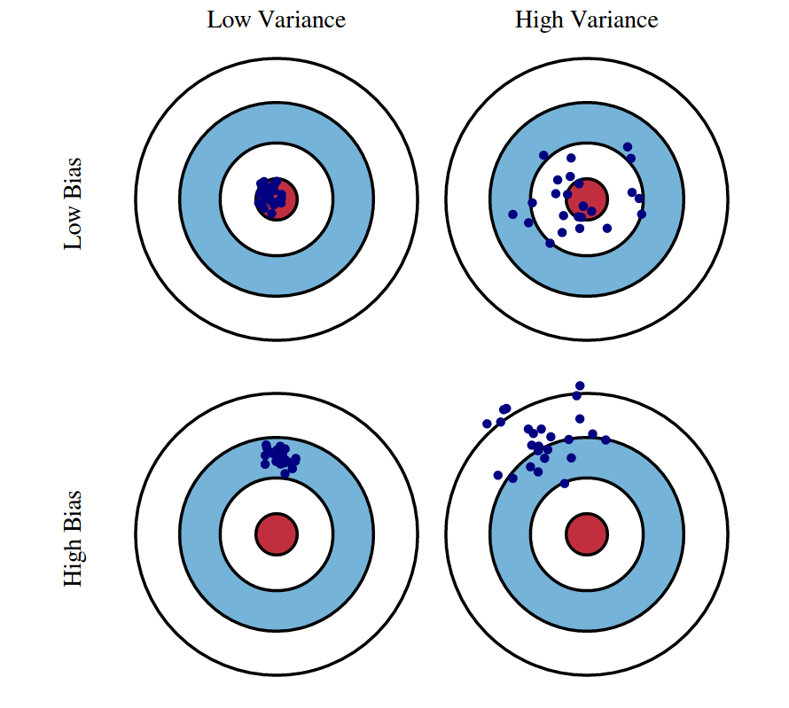
- Variance: Literally, it is how much our classifier on training data deviates from the expected classifier. This value captures how much your classifier changes if you train on a different training set. How “over-specialized” is your classifier to a particular training set (overfitting)?
- Bias: Literally, this is how much error the best classifier still makes. It captures the inherent error that you obtain from your classifier even with infinite training data. This is due to your classifier being “biased” to a particular kind of solution (e.g. linear classifier). In other words, bias is inherent to your model and dependent on the algorithm .
- Noise: How big is the difference between the test point’s label and the expected label? This is a data-intrinsic noise that measures ambiguity due to your data distribution and feature representation. You can never beat this, it is an aspect of the data.
Fig 1: Graphical illustration of bias and variance. If we have bias, it will be the board constantly shaking, so you can hardly ever hit it.
Detecting High Bias and High Variance
If a classifier is under-performing (test or training error is too high), the first step is to determine the root of the problem.
Figure 3: Test and training error as the number of training instances increases.
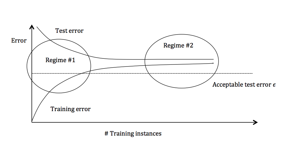
The graph above plots the training error and the test error and can be divided into two overarching regimes. In the first regime (on the left side of the graph), training error is below the desired error threshold (denoted by ), but test error is significantly higher. In the second regime (on the right side of the graph), test error is remarkably close to training error, but both are above the desired tolerance of .
Regime 1 (High Variance)
In the first regime, the cause of the poor performance is high variance.
Symptoms:
- Training error is much lower than test error
- Training error is lower than
- Test error is above
Remedies:
- Add more training data
- Reduce model complexity, usually by adding a regularization term (complex models are prone to high variance)
- Bagging (will be covered later in the course)
- Early Stopping
Regime 2 (High Bias)
Unlike the first regime, the second regime indicates high bias: the model being used is not robust enough to produce an accurate prediction.
Symptoms:
- Training error is higher than
Remedies:
- Use more complex model (e.g. kernelize, use non-linear models)
- Add features
- Boosting (will be covered later in the course)
Thought Process to determine whether a model is high bias / variance:
- High Variance:
- Imagine you train several models on different dataset you draw from the original distribution , each dataset is very small. How do the results compare with each other? If differ by a lot, high var.
- Is this model overfitting? If yes, high var.
- High Bias:
- Imagine you train this model on all data from the original distribution , if it still performs badly, it has a high bias.
- Is this model underfitting? If yes, high bias.
Example:
| Bias | Variance | |
|---|---|---|
| kNN with small k | low | high |
| kNN with large k | high | low |
Ideal Case
Training and test error are both below the acceptable test error line.
Reduce Noise
Two reasons can cause noise and we introduce the corresponding solution:
- Labels are just wrongly assigned <- no solution but to assign the correct label
- Features are not expressive enough <- add more features